Electrical Simulations of Series and Parallel PV Arc-Faults. Jack Flicker and Jay Johnson. Sandia National Laboratories, Albuquerque, NM 87185, USA.
Electrical Simulations of Series and Parallel PV Arc-Faults Jack Flicker and Jay Johnson Sandia National Laboratories, Albuquerque, NM 87185, USA Abstract—Arcing in PV systems has caused multiple residential and commercial rooftop fires. The National Electrical Code® (NEC) added section 690.11 to mitigate this danger by requiring arc-fault circuit interrupters (AFCI). Currently, the requirement is only for series arc-faults, but to fully protect PV installations from arc-fault-generated fires, parallel arc-faults must also be mitigated effectively. In order to de-energize a parallel arc-fault without module-level disconnects, the type of arc-fault must be identified so that proper action can be taken (e.g., opening the array for a series arc-fault and shorting for a parallel arc-fault). In this work, we investigate the electrical behavior of the PV system during series and parallel arc-faults to (a) understand the arcing power available from different faults, (b) identify electrical characteristics that differentiate the two fault types, and (c) determine the location of the fault based on current or voltage of the faulted array. This information can be used to improve arc-fault detector speed and functionality. Index Terms—SPICE, series and parallel arc faults, PV, AFD, AFCI
I. INTRODUCTION National Electrical Code® 690.11 only requires series arcfault protection for PV systems [1]. This leaves the possibility of a parallel arc-fault establishing a fire. As a result, UL 1699B [2] provides a testing protocol for listing a Type 2 device capable of mitigating series and parallel arc-faults, and the PV industry is currently pursuing parallel arc-fault detection, differentiation, and mitigation techniques [3-5]. MidNite Solar, Inc. has developed the first series and parallel AFCI combiner box prototype, which first assumes a series arc-fault when there is arc-fault noise on the array and opens the string(s); then the AFCI rechecks for arcing noise and shorts the array to de-energize the parallel arc-fault if necessary. However, there are many alternative approaches to detecting and differentiating series and parallel arc-faults presented in previous work [3]; the simplest of which would be to monitor the high frequency noise created by the arc-fault in conjunction with the current and voltage of the array. Numerical and experimental studies were performed to determine the accuracy and robustness of using this method for a range of fault types, impedances, and locations. Differentiating series and parallel arc-faults is important if the interrupting devices (IDs) of the Type 2 arc fault circuit interrupter (AFCI) are not located at each module. If the Type 2 AFCI is at the combiner or inverter, the arc-fault protection system must open the array if there is a series arc-fault and short the array if there is a parallel arc-fault. Unfortunately, if the wrong action is taken, the arc will continue and the fault power will increase.
To better understand the different fault types and determine if there is a surefire method of differentiating the faults, Sandia National Laboratories (SNL) has developed a PV array model [6] using a simulation program with integrated circuit emphasis (SPICE) [7]—a free node-based electrical modeling software—to better understand the electrical dynamics of the series and parallel arc-faults. The SPICE models of different arc-faults have been studied in hopes of creating a quick, accurate differentiation scheme between different types of parallel and series arc-faults using current/voltage information that is already being collected by the inverter during PV array operation. In order to validate the SPICE model, a number of the simulated faults were compared to field experimental studies performed at the Distributed Energy Technologies Laboratory (DETL) at SNL using both a set of power resistors—which simulated solid ground faults, line-line faults, and increased series resistance in the PV string from damage or corrosion— and an arc-fault generator (AFG) similar to the one used in UL 1699B [4] to simulate: 1. series arc-faults in the string, 2. intra-string parallel arc-faults, 3. cross-string parallel arc-faults, and 4. arcing ground faults To validate the inverter model and eliminate the transient dynamics of the inverter, a variable load bank surrogate was used and set to the maximum power point (MPP) of the unfaulted array. Therefore, all the fault types were conducted with all the combinations of load bank/inverter and resistor/AFG. The resistor situations with an inverter are shown in Figure 1. Note that the ground fault simulations were conducted by faulting to the grounded current carrying conductor as opposed to the equipment grounding conductor because the electrical behavior of the array is nearly the same and it would not clear the ground fault fuse. Experiments and simulations were performed in parallel for the different test cases in the following order: 1. Resistance faults with the load bank were studied to find SPICE parameters for the PV modules and provide a baseline for the other tests. 2. Arc-faults with the load bank were studied to ensure the SPICE arc-fault model (a resistor) accurately simulated the dynamic electrical behavior of arc plasmas. 3. Numerical and experimental studies of solid ground faults, series faults, and line-line faults were used to analyze the behavior of faulted PV systems with an inverter.
4.
Experimental tests and simulation-based verification of different arc-faults was used to determine the type and location of the fault. String 2
String 1
High Impedance Series Fault [Series Arc-Fault]
7+
7+
7
7 6+
6 5+
c
Intra-string Line-Line Fault [Intra-string Parallel Arc-Fault]
5
6+
Inverter
5+
~
6
5 4+
4+
4 3+
Cross-string Line-Line Fault
3+
c
3
[Cross-string Parallel Arc-Fault]
GFPD
4
3 2+
2+
2
Ground Fault [Arcing Ground Fault]
2
The PV array model is comprised of two strings wired in parallel. Each string is composed of seven modules in series. Each module is connected to a bypass diode (Io=4.7·10-12 A, N=1). For the purposes of simulation, the fault location is denoted by “n+” notation, where n+ indicates the fault position at the positive terminal of the nth module above the grounded CCC. In each simulation, the PV array is constructed with multiple modules connected to a central load that approximates the impedance of the inverter or load bank used in the experimental conditions. The arc-fault is modeled by a simple resistor with the resistance determined by the ratio of the measured median arc voltage to the median arc current for each fault scenario. The results from the constant resistance fault with a load bank were used to generate the PV module parameters for the simulations. The model errors are shown in Fig. 2 for the different fault types. The fault errors are often larger than the array errors because of the small values and measurement error.
1+
1+
1
1 Grounded Current Carrying Conductor (CCC)
Equipment Grounding Conductor (EGC)
Fig. 1. Different types of series and parallel solid faults (blue) and arc-faults (red, bracketed) on the DC side of a PV array composed of two strings.
II. PV MODEL Computer circuit simulations are able to model non-linear PV circuits for a wide variety of conditions [8]. A common method of circuit simulation is the use of SPICE. In this work, MacSPICE is used to analyze the behavior of a PV array during various arc-fault conditions [9, 10]. The SPICE model of the PV array uses a single module as the base building block. The construction of a single module is accomplished using a standard one-diode model [6]. This model consists of an ideal current source with a value equal to the module short-circuit current (Isc) in parallel with a diode and shunt resistance (Rsh) all in series with a series resistance (Rs). In order to increase the Voc of the module above the voltage drop of a regular diode (~0.6 V), the ideality constant of the diode (N) must be increased [9]. The one-diode model was constructed to approximate the IV curve of 200 W monocrystalline Si modules located at DETL. The parameters of the one-diode model change for each simulation to account for changes in solar irradiance and module operation temperature. For an irradiance of 900 W/m2, the current source is set to supply 3.2 A at short circuit (SC), the diode has an ideality factor of N=131 and leakage current Io=2.85·10-8 A, Rsh is set 550 Ω and the Rs is set to 900 mΩ. This module gives an IV curve with Isc of 3.2 A, Voc of 63.24 V, and Pmp of 137.5 W. The max power point (MPP) has Imp=2.67 A and Vmp=51.5 V.
Fig. 2.
Model errors for the resistor fault and load bank.
III. THEORETICAL DIFFERENTIATION OF ARC-FAULT TYPES AND FAULT FINDING The primary goals of the simulations are to (a) determine the type of arc-fault (series vs. parallel) using measurements at the inverter (array current and voltage) so that proper deenergization procedures (opening or shorting) can be performed and to determine where arc-faults occurred using the IV curve of the array. Note that after a series arc-fault has been mitigated, the burned/damaged conductor will likely be open and easily located, but after a parallel arc-fault, there may be no change in the array IV curve because there is no longer a conduction path between the parallel conductors. Therefore, determining the location of the parallel arc-fault would have to be performed while the arc existed. However, these techniques could be used to locate line-line faults. A. Series arc-faults Ideal PV arrays have near zero impedance in module interconnects and connectors. Series faults occur due to degradation in solder joins, PV wiring, or junction boxes, increasing the interconnect impedance above its nominal
value. These faults and series arc-faults act much like an increase in Rs in a specific module [11]. For a small increase in impedance, both array Isc and Voc are unchanged, while the fill factor of the array IV curve decreases (Fig. 3). As the interconnect impedance increases above ~60 Ω, the array Isc monotonically decreases while the array Voc remains unchanged. Experimental series arc-faults had resistance values between 5-25 Ω, however, so there were only slight changes to the IV curve of the array.
Fig. 3. curve
B. Parallel arc-faults Parallel arc-faults come in three varieties: cross-string, intra-string, and ground. These faults are especially dangerous since (unlike series arc-faults) a pathway exists for fault current to flow even when the array is open, posing both a fire and shock hazard. In each type of parallel arc-fault/line-line, the symmetry of the array is altered and the faulted string appears to be composed of fewer modules than in the unfaulted case. This has the effect of decreasing the Voc proportional to the number of modules while leaving Isc unaffected, shown in Fig. 6. Parallel arc-faults that bypass different numbers of modules are relatively easy to differentiate from each other due to the large changes in Vmp and Voc. The differentiation between fault types that bypass the same number of modules is slightly more complex. It is not possible to resolve the location of intra-string parallel arc-faults or arcing ground faults from either the array current or voltage. This is because the IV curve of a faulted string is identical regardless of which module is faulted (Fig. 7) and is dependent only on the fault impedance and number of modules bypassed.
Effect of series fault of different impedances on array IV
For series arc-faults, the IV curve of the array is independent of the location of the series fault so this method cannot be used to determine the fault location (Fig. 4), but an IV curve could be used to estimate fault impedance using Isc or fill factor (FF) as an indicator (Fig. 5).
Fig. 6. Cross-string parallel faults (2nd string module location designated with the ‘B’) decrease array Vmp and Voc. This decrease is a linear function of the number of modules bypassed by the fault and the same for intra-string arc-faults and arcing ground faults.
Fig. 4. Series faults at different locations of the array cause identical effects on the array IV curve and, therefore, cannot be resolved
Fig. 5. Series fault impedance affects both array FF and the Isc of the shorted string. These parameters can be used to estimate the fault impedance
Fig. 7. Intra-string faults impact the array IV curve similarly, making it impossible to discern their location from array electrical measurements. This behavior exists for ground faults and intra-string line-line faults as well [10].
Unlike intra-string faults, the location of cross-string faults is identifiable if precision measurements of the IV curve are possible. The Voc of a PV array under a cross-string fault does depend slightly on the position of the fault (Fig. 8) due to module non-idealities in the current pathway (most likely added values of Rsh). Unlike the intra-string fault, where the unfaulted string IV curve is identical before and after the fault, in a cross-string fault, both strings are effected; and due to the presence of series resistance in the modules, this changes the Voc for the two strings and yields a slight mismatch dependent on fault position.
IV. EXPERIMENTAL ARC-FAULT TESTS AND MODEL VALIDATION In order to validate the SPICE model and expand on the work in [6], a series of arc-fault tests were performed on real PV arrays at DETL composed of two parallel strings of seven 200 W monocrystalline Si modules connected in series. In each experiment, the fault was installed between modules using MC4 T-branch connectors. The fault and array current and voltage were collected with a Tektronix DPO3014 oscilloscope, two Tektronix P5200 differential voltage probes, and two Tektronix TCP303 current probes. A. Constant resistance fault with load bank The PV array was connected to a load bank with impedance (55.6 Ω) approximately equal to the array MPP and resistive faults of 3.2, 5.1, 10.5, and 22.4 Ω were established for each of the fault types. To calibrate the SPICE model to the unfaulted array and to validate the model for the faulted array, IV curves were taken of the array using a Daystar, Inc DS100C IV curve tracer. The model closely predicted the IV curve for intra-string faults, such as the 2+ to 1+ example shown in Fig. 10.
Fig. 8. Cross-string faults impact the array Voc differently depending on fault location in the array. The position of the cross-string fault can, theoretically, be determined through electrical measurements.
C. Differentiation of Series, Intra-, and Cross-string Faults The range of fault types, locations, and impedances, make it difficult to differentiate between series and parallel arc-faults based purely on array IV behavior. Depending on the exact meteorological conditions, each fault could have nearly the same effects on the array IV curve, especially at MPP (Fig. 9). Therefore, based on the steady-state SPICE model, differentiation between series and parallel faults cannot be achieved through current and voltage measurement at the inverter.
Fig. 9. Without knowing either the type of fault or fault impedance, it may be difficult to determine both from electrical measurements since they have similar effects on the array IV curve.
Fig. 10. Experimental IV curves of faulted and unfaulted states (solid lines) overlaid with SPICE simulations (dots).
Fig. 11 shows the results of array current and voltage for the four different faults with the 5.1 Ω resistor and load bank. The array current and voltage shows a linear dependence on number of modules faulted, nearly independent of fault type (differences are most likely due to changing environmental conditions such as irradiance and temperature), as predicted by theory (Fig. 6). The solid line denotes the load bank line (55.6 Ω). The fault impedance controls the spacing of points along the line. High impedance faults lie close together at high voltage and current values since those faults yield smaller drops in faulted array voltage and current. Low impedance faults are spread farther out along the load line. Fig. 12 shows the results of experimental ground fault tests of the PV array using the resistors. The top figure shows fault current/voltage information. The dashed lines indicate the different resistances used for the faults. The bottom figure shows excellent correlation between array current/voltage
information for the experiments and SPICE simulations. The dashed line shows the load bank impedance (55.6 Ω).
Fig. 11. Results of faulted array current and voltage for various types of faults for a fault impedance of 5.1 Ω.
resistance faults, arc-fault experimental data was compared to the simulations. As opposed to a constant resistance, arc faults have a time-variable, current-dependent resistance. The arc-faults were generated using the procedure highlighted in [12]. For the purposes of simulation, the arc resistance was calculated using the ratio of the measured arc voltage and current. The results of the experimental tests and corresponding SPICE simulations are shown in Fig. 13 for ground faults, series faults, cross-string faults, and intra-string faults. The SPICE simulations match well with the experimentally collected data points (