Index Terms â Wavelet neural networks, ECG signal, particle ... remove high frequency noise from ECG signal is to employ a low-pass filter [9]. However, the ...
Proceedings of the IEEE International Conference on Automation and Logistics Shenyang, China August 2009
Electrocardiogram (ECG) Signal Modeling and Noise
Reduction Using Wavelet Neural Networks*
Suranai Poungponsri, Xiao-Hua Yu Department of Electrical Engineering
California Polytechnic State University
San Luis Obispo, CA 93407, USA
remove high frequency noise from ECG signal is to employ a low-pass filter [9]. However, the cut-off frequency is difficult to determine and it may introduce some additional artifacts to the signal, especially on the QRS wave. Other filtering techniques that have been proposed concentrate on the design of hybrid filters and filter banks, such as [10]. The concept of Wavelet Neural Network (WNN) was inspired by both the technologies of wavelet decomposition and neural networks. In standard neural networks, the inputoutput mapping is approximated by the superposition of sigmoid functions; while in WNN, this relationship is approximated by the superposition of a series of wavelet functions. WNN combines the multi-resolution nature of wavelets and the adaptive learning ability of neural networks, and has found many applications in time series prediction, function approximation and fault diagnosis. In this research, WNN is studied for ECG signal modeling and noise reduction. The network is trained by a hybrid algorithm with ADLPSO (Adaptive Diversity Learning Particle Swarm Optimization) and gradient descent optimization. Computer simulation results demonstrate this proposed approach can successfully model the ECG signal and remove high-frequency noise.
Abstract - Electrocardiogram (ECG) signal has been widely used in cardiac pathology to detect heart disease. In this paper, wavelet neural network (WNN) is studied for ECG signal modeling and noise reduction. WNN combines the multiresolution nature of wavelets and the adaptive learning ability of artificial neural networks, and is trained by a hybrid algorithm that includes the Adaptive Diversity Learning Particle Swarm Optimization (ADLPSO) and the gradient descent optimization. Computer simulation results demonstrate this proposed approach can successfully model the ECG signal and remove high-frequency noise. Index Terms – Wavelet neural networks, ECG signal, particle swarm optimization.
I. INTRODUCTION The electrocardiogram (ECG) signal is generated by the rhythmic contractions of the heart. It represents the electrical activity of the heart muscles, and is usually measured by the electrodes placed on body surface. Clinical data show that ECG signal is very effective to detect heart disease. A typical one cardiac cycle ECG waveform which consists of a P-wave, a QRS-complex, and a T-wave, is shown in Fig. 1.
II. THE WAVELET NEURAL NETWORK AND LEARNING ALGORITHM In wavelet transform, various wavelets are generated from a single basic wavelet ψ ( t ) known as the mother wavelet. This is done by introducing the scale (or dilation) factor, s; and translation (or shift) factor, τ . The shifted and dilated versions of the mother wavelet can be expressed as: Fig. 1. A typical ECG signal
ψ s ,τ ( t ) =
It should be noticed that even though the ECG signals from different patients have the similar forms, the ECG of each individual patient is different. To make appropriate medical diagnosis, doctors often need to compare the ECG signal with the patient’s own individual record. Therefore, modeling the ECG signal for each patient becomes very important in clinic practice. In addition, ECG signal is often corrupted with noise, which makes an accurate diagnosis very difficult. ECG noise removal is complicated due to the timevarying nature of ECG signals. The traditional approach to *
1 s
⎛ t −τ ⎞ ⎟ ⎝ s ⎠
ψ ⎜
The wavelet transform of a signal x(t) with mother wavelet function ψ ( t ) can be written as:
T( s,τ ) =
1
s∫
∞
−∞
⎛ t −τ ⎞ x( t ) ψ * ⎜ ⎟ dt ⎝ s ⎠
(2)
The asterisk indicates that the complex conjugate of the wavelet function is used in the transform. In fact, wavelet transform can be thought of as the cross-correlation of a signal with a set of wavelets of various “widths.”
This work was supported in part by the Department of the Navy, Office of Naval Research, under Award # N00014-08-1-1209.
978-1-4244-4795-4/09/$25.00 © 2009 IEEE
(1)
394
A typical Wavelet Neural Network (WNN) contains an input layer, an output layer, and a hidden layer. It employs a set of wavelets as the activation functions of the hidden neurons. Fig. 2 shows the structure of a WNN with multiple inputs x1 , x2 , …, xn , where Ψi (i = 1, 2, …, N) represents
preset fitness criterion, it is recorded as p i . When a particle takes all the population as its topological neighbors, the best neighbor solution becomes a global best and is called p g . In the particle swarm optimization algorithm, the velocity v of particle i moving toward its local p i and global optimal locations is updated at each training step. It is weighted by the two terms ( φ1 and φ2 ) that are randomly distributed in [0, 1]
the wavelet function of each hidden neuron; and g is the bias of the output neuron.
with two separate constant coefficients c1 and c2 (in general, the range of c1 and c2 is [0, 4]). That is,
vi ( k + 1 ) =
χ [αvi ( k ) + c1φ1 ( p i ( k ) − z i ( k )) + c2φ 2 ( p g ( k ) − z i ( k ))] (4) where i = 1, 2, …, N T and N T is the total number of particles (i.e., population size); χ and α are two real constant coefficients; and k is the index of generation. The parameter χ controls the magnitude of v, whereas the inertial weight α
Fig. 2. The Wavelet Neural Network
For this application, we choose the mother wavelet function to be the following:
ψ ( x ) = −x
weights the magnitude of the old velocity vi ( k ) in the calculation of the new velocity vi ( k + 1 ) . Based on the updated velocity, each particle changes its position according to the following equation: z i ( k + 1 ) = z i ( k ) + vi ( k + 1 ) (5) The idea of Adaptive Diversity Learning PSO (ADLPSO) was introduced ([2]) to avoid the tendency of “localized cluster” in the PSO algorithm. In PSO algorithm, when a local optimum is found by one particle, the other particles will be drawn toward it. In other words, all particles may tend to stay at the same local optimum without much chance to escape. The basic idea of Adaptive Diversity Learning (ADL) is to allow some of the particles explore other areas in the solution space for possible better solutions. ADL is actually integrated as an additional part in PSO. In each generation, the performances of all particles are evaluated and ranked by a fitness rule. The particles are then divided into two groups. The first group contains most of the particles (usually about 70% of the total population) with “good” performance while the second group contains a relatively smaller portion of particles (usually about 30% of the total population) with the “not-so-good” performance. All the particles in group-one are updated by the basic PSO algorithm (using Eq. (4) and (5)); the particles in group-two, however, are enhanced by a diversity model (ADL). Let the total number of particles of the second group (i.e., the one updated by ADL) be denoted by N s ; and note that
1 − x2 e 2
(3) The plot of the mother wavelet function can be found in Fig. 3, which yields a similar shape as the ECG signal shown in Fig. 1. 0.8 0.6 0.4 0.2 0 -0.2 -0.4 -0.6 -0.8 -8
-6
-4
-2
0
2
4
6
8
Fig. 3. The Mother Wavelet Function
The Particle Swarm Optimization (PSO) is a population based optimization method first proposed by Kennedy and Eberhart ([1]) in 1995. PSO is a multi-agent parallel search technique, inspired by the social behavior of bird flocking or fish schooling. It shares many similarities with evolutionary computation techniques such as Genetic Algorithm (GA). Both of them are initialized with a population of random solutions; then both algorithms search for optima, and update their solutions in each generation. However, unlike GA, PSO has no evolution operators such as crossover and mutation. In PSO, the potential solution is the optimum particle of the current generation that flies through the multi-dimensional search space. Each particle keeps track of its coordinates (represented by a position vector zi ) in the space. If a best solution (among its neighborhood) can be found based on a
N s ≤ N T . According to [2], the diversity model can be specified using a specific probability density function (PDF): βx ⎪⎧(1− q ) β e p( x ) = ⎨ −β x ⎩⎪q β e
395
x≤0 x>0
(6)
Thus, a random diversity vector can be written as:
[
~ d = d1 ,d 2 ,",d N s
]
where n is the total number of inputs of the neural network. For a real mother wavelet function, substituting Eq. (1) into Eq. (10), we obtain:
(7)
Each element in the vector can be found as:
⎧ 1 ⎛ ri ⎞ ⎟⎟ ,
⎪ ln⎜⎜ ⎪ β ⎝ 1 − qi ⎠
d i = ⎨
⎪ 1 ⎛⎜ 1− ri ⎞⎟ ⎪− β ⎜ q ⎟ ,
⎩ ⎝ i ⎠
∑ (w Ψ ( ~ x )) + g
0 < ri ≤ (1 − qi )
~ x = ( x1 ,x2 ," ,x n ) ~ τ i = ( τ i ,1 ,τ i ,2 ,",τ i ,n ) ~s = ( s ,s ,",s ) i
i ,2
i,n
d ψ ( ~x ) ~ d x
~ ~
~z = xk − τ i i ~s
(14) (15) (16)
(17) (18)
i
Also, let J k , the objective function of the k th training iteration, be the square error:
(9)
1 J k = ( ek ) 2 2
th
of iterations (in the k generation). Similar to the basic PSO, ADL updates the particle positions using the following rule:
(19)
where
ek = g θ ( ~ x ) − yk
(20) Then by using chain rule, the gradient of each parameter can be calculated as:
(10)
dJ k = ek dg dJ k = ek Ψ ′( ~z i ) dwi
ADLPSO is a very effective global search algorithm; however, it may not be able to find an accurate solution. On the other hand, gradient descent algorithm is capable of finding a precise solution within certain rage, but it may be easily trapped in local minimum. In this research, a hybrid algorithm ([2]) is employed to train WNN. A region in search space is located by ADLPSO first; then the gradient descent algorithm is used to fine-tune the optimum solution in this region. Note that in Fig. 2, for each wavelet function of a hidden neuron, two more parameters (i.e., the scale factor and the translation) must be considered (in addition to the weights of NN). Let the NN output (single output) be:
(21) (for multiple inputs)
or
dJ k = ekψ ′( ~z i ) dwi
N
(11)
(for single input)
(22)
⎛1⎞ dJ k = − ek wi ⎜⎜ ~ ⎟⎟ψ ' (~zi ) ~ dτ ⎝ si ⎠
(23)
⎛ 1 ⎞
dJ k = − ek wi ⎜⎜ ~ 2 ⎟⎟(~ xk − τ~i )ψ ' (~z i ) ~ ds s ⎝ i ⎠
(24)
Finally, each parameter is updated as:
i=1
dJ k dg dJ wi ( k + 1 ) = wi ( k ) − η k dwi
th
where wi is the weight (connection) from the i neuron in the hidden layer to the output; and N is the total number of neurons in the hidden layer. For a multivariate wavelet basis function, it can be calculated by the tensor product of single wavelet basis function as follows:
g( k + 1 ) = g( k ) − η
τ~( k + 1 ) = τ~( k ) − η
n
∏ψ ( xi )
i ,1
ψ ′( ~x ) =
where t is the index of iteration and T is the maximum number
Ψ( ~ x )=
(13)
For simplicity, let
the k th generation) is performed more than once, then β can be updated in each iteration:
T
⎞⎞ ⎟⎟ ⎟ + g ⎟
⎠ ⎠
where
search direction. The larger the qi , the higher search probability in positive direction. Another control parameter β determines the range of the diversification search. The larger the β, the smaller range of local search. If this local search (in
[β ( k ) − β ( 0] ( T − t ) + β ( 0 ) β ( k +1) =
~ ⎛ ~ − 1 ⎛ ~ ⎜ wi si 2 ψ ⎜ x − τ i ⎜ ~
⎜
⎝ si i=1 ⎝
∑
where i = 1, 2, …, N s ; ri is a real random number uniformly distributed between [0, 1]. Note that we search around the local area in both positive and negative direction. The adjustable parameter qi ∈ [0,1] determines the probability of
∑ (wi Ψi ( x )) + g
i
N
=
( 1 − qi ) ≤ ri < 1
g( x ) =
i
i=1
(8)
~z ( k + 1 ) = ~z ( k ) + d~( k + 1 ) ~ where d ( k + 1 ) can be calculated by Eq. (8).
N
g( ~ x ) =
(12)
i=1
396
dJ k dτ~
(25) (26) (27)
dJ ~s ( k + 1 ) = ~ s ( k ) − η ~k ds
shown in (c). Obviously, the traditional filter can eliminate some, but not all the noise in the signal.
(28)
where η is the learning rate. The flow chart of the overall training algorithm is shown in Fig. 4.
Noisy-free ECG
2
1
0
-1
4000
4500
5000
5500
6000
6500
7000
7500
8000
6500
7000
7500
8000
Noisy ECG
2
1
0
-1
4000
4500
5000
5500
6000
(a) 2.5
2
1.5
Fig. 4. The ADLPSO-Gradient Training Algorithm
1
0.5
0
III. SIMULATION RESULTS
-0.5
In this section, the proposed wavelet neural network (trained by the adaptive diversity learning particle swarm optimization and the gradient descent algorithm) is applied to ECG signal modeling and noise reduction. Both training and testing data are taken from [5]. White noise is added to the original (clean) ECG signal and the SNR (signal to noise ratio) of the noisy (unfiltered) signal is about 17.7dB. The neural network is trained using noisy ECG data as its input, with clean (noise-free) signal as the desired target. In the hybrid algorithm, the neural network is trained by ADLPSO with 400 iterations first, then trained by the gradient descent algorithm by 1600 iterations. The number of population is 20. The simulation results are shown in Fig. 5. The ECG signals are shown in (a), with the clean (noise-free) signal on the top and the noisy signal on the bottom. The output of NN (in (b)) is smoother than the input, indicating that a welltrained WNN can effectively filter out high frequency noise. The SNR of the filtered signal (i.e., the output of NN) is approximately 21.1dB (or 4.1dB of improvement). In general, for diagnostic purpose, the range of interest of
ECG signal is about 0.05 Hz at the lower end of spectrum
which allows for ST segments to be recorded and 40, 100, or
150 Hz in the higher end spectrum [8]. The choice for the
frequency at the higher end depends on the patient’s health
and profile conditions as well as what type of diagnostic a
doctor wants to capture. To compare the result of WNN with
the traditional approach, a 501-tapped FIR low-pass filter with
cut-off frequency at 90Hz is employed. The filtered signal is
397
-1
-1.5 4000
4500
5000
5500
6000
6500
7000
7500
8000
6500
7000
7500
8000
(b)
2.5
2
1.5
1
0.5 0 -0.5 -1 -1.5 4000
4500
5000
5500
6000
(c) Fig. 5. Neural Network Testing Results
(a) The clean (Noise-free) signal (top) and the unfiltered noisy (bottom)
(b) The filtered ECG signal (by NN, solid line) and
the clean signal (dotted line)
(c) The filtered ECG signal (by low-pass filter, solid line) and
the clean signal (dotted line)
IV. CONCLUSIONS An approach to study ECG signal based on wavelet neural network and adaptive diversity learning particle swarm optimization algorithm for network training is investigated in this paper. Computer simulation results show this approach is promising for ECG signal modeling and noise reduction. More tests will be conducted to further investigate its performance in the future. REFERENCES [1] J. Kennedy and R. Eberhart, “Particle swarm optimization,” Proc. IEEE Int. Conf. Neural Networks, pp.1942-1948, 1995. [2] Y. Chen, B. Yang, and J. Dong, “Time-series prediction using a local linear wavelet neural network,” Neurocomputing, vol. 69, pp.449-465, 2006. [3] Q. Zhang, and A. Benveniste, “Wavelet networks”, IEEE Trans. Neural Network, Vol. 3, No. 6, p.889-898, 1992 [4] S. Haykin, Neural Networks: A Comprehensive Foundation, 2nd ed., Prentice Hall, 1999. [5] PhysioBank, The MIT-BIH noise stress test database, http://www.physionet.org/physiobank/database/nstdb/. [6] PhysioBank, MIT-BIH arrhythmia database, http://www.physionet.org/physiobank/database/mitdb/. [7] G. Moody, WFDB applications guide, http://www.physionet.org/physiotools/wag/nst-1.htm#sect4. [8] Wikipedia, “Electrocardiogram”, http://en.wikipedia.org/wiki/ECG. [9] T. Slonim, M. Slonim, E. Ovsyscher, “The use of simple FIR filters for filtering of ECG signals and a new method for post-filter signal reconstruction”, Proc. Computers in Cardiology, 1993. [10]V. Afonso, W. Tompkins, et al., “Filter bank-based processing of the stress ECG,” IEEE 17th Annual Conference on Engineering in Medicine and Biology Society, 1995.
398