Electromagnetic Brain Mapping using MEG & EEG1

Electromagnetic Brain Mapping using MEG & EEG

1

Sylvain Baillet

Department of Neurology, Medical College of Wisconsin Milwaukee, USA

Abstract

Electroencephalography (EEG) and magnetoencephalography (MEG) are techniques dedicated to the non-invasive detection of neural current ows through the electromagnetic eld they generate and that can be measured outside the head. Though MEG and EEG were born in physics and electrophysiology laboratories several decades ago, they have constantly evolved by integrating new technological and methodological advances. In the neuropsychology lab, EEG has rapidly been adopted as a technique to investigate the timing and scalp topography of specic brain responses elicited by a stimulus. Today, MEG and EEG set-ups integrate from several dozens to hundreds of sensors distributed outside the head, which once combined with models of electromagnetics within brain and head tissues allow the estimation of the neural generators of these `brain waves'. This has given rise to techniques for time-resolved electromagnetic brain mapping, which this chapter reviews in more details with a pragmatic standpoint, and an emphasis on the experimental benets of accessing brain activation at the millisecond time scale. Keywords: neuroimaging; techniques & methods; event-related brain responses; neural oscillations; evoked potentials & elds; induced brain activity; ongoing brain activity; brain networks; coherence & synchrony; functional connectivity.

Introduction

Accessing brain activity non-invasively using neuroimaging techniques has been possible for about two decades and has continued to thrive from the technical and methodological standpoints (K. J. Friston, 2009). With the ubiquitous availability of magnetic resonance imaging (MRI) scanners in major hospitals and research centers, functional-MRI (fMRI) has certainly become the modality-of-choice to approach the human brain in action. A welldocumented and thoroughly-discussed limitation of fMRI however, sits in the very physiological origins of the signals accessible to the analysis. Indeed, fMRI is essentially sensitive 1 For publication in: Handbook of Social Neuroscience, eds: Jean Decety & John Cacioppo, Oxford University Press (2010).

ELECTROMAGNETIC BRAIN MAPPING

2

to local uctuations in blood oxygen levels and ow, which connexion to cerebral activity is the object of very active scientic investigations and sometimes, controversies (Logothetis & Pfeuer, 2004; Logothetis & Wandell, 2004; Eijsden, Hyder, Rothman, & Shulman, 2009). A more fundamental limitation of fMRI and metabolic techniques such as Positon Emission Tomography (PET) is the lack of temporal resolution. In essence, the physiological changes captured by these techniques uctuate within a typical time scale of several hundreds of milliseconds at best, which makes them excellent at mapping the regions involved in task performance or resting-states (Fox & Raichle, 2007), but incapable of resolving the ow of rapid brain activity that unfolds with time. Metaphorically speaking, metabolic and hemodynamic techniques perform as very sensitive cameras that are able to capture low-intensity signals using long aperture durations, hence a sluggish temporal resolution. This basic limitation has become salient as new neuroscience questions emerge to investigate the brain as an ensemble of complex networks that form, reshape and ush information dynamically (Varela, Lachaux, Rodriguez, & Martinerie, 2001; Sergent & Dehaene, 2004; Werner, 2007). An additional, though seemingly minor, limitation of these modalities consist in their operational environment: most scanners are installed in hospitals, with typically limited access time but more importantly, necessitate that subjects lie supine in a narrow tunnel, with loud noises generated by the acquisition processes. Such non-ecological environment is certainly detrimental to the subject's comfort and therefore, limits the possibilities in terms of stimulus presentation and real-time interaction with participants, which are central issues in Social Neuroscience studies. This chapter therefore describes how Electroencephalography (EEG) and Magnetoencephalography (MEG) oer complementary alternatives to typical neuroimaging studies in that respect. We will briey review the basic, though very rich, methods of sensor data analysis, which focus of the chronometry of so-called brain events. We will further emphasize how MEG and EEG may be utilized as neuroimaging techniques, that is, how they are capable to map dynamic brain activity and functional connectivity with fair spatial resolution and unique rapid time scales. EEG recordings have been made possible in the MRI environment, therefore leading to multimodal data acquisition and analysis (Laufs, Daunizeau, Carmichael, & Kleinschmidt, 2008). This has brought up interesting discussions and results on e.g., rapid phenomena such as epileptiform events and the electrophysiological counterpart of BOLD resting-state uctuations (Mantini, Perrucci, Gratta, Romani, & Corbetta, 2007). MEG and EEG data acquired with high-density sensor arrays also stand by themselves as functional neuroimaging techniques: this is the realm of electromagnetic brain mapping (Salmelin & Baillet, 2009). It is indeed interesting to note that MEG instruments are being delivered to prominent functional neuroimaging clinical and research centers who are willing to expand their investigations beyond the static, functional cartography of the brain. This chapter oers a pragmatic review of this rapidly evolving eld. MEG/EEG Principles and Instrumentation

Physiological sources of electromagnetic elds All electrical currents produce electromagnetic elds, and our body is inundated by currents of all sorts. The muscles and the heart are two well-known and strong sources of electrophysiological currents, qualied as ànimal electricity' by early scientists like Luigi


3

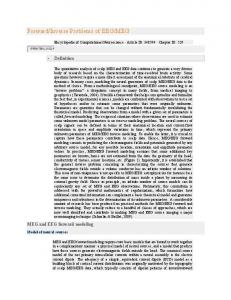
Galvani, who were able to evidence such phenomena more than 200 years ago. The brain also sustains ionic current ows within and across cell assemblies, with neurons as the strongest generators. The architecture of the neural cell as decomposed into dendritic branches and tree, soma and axon conditions the paths taken by the tiny intracellular currents owing within the cell. The relative complexity and large variety of these current pathways can be simplied by looking at the cell from some distance: indeed, these elementary currents instantaneously sum into a net primary current ow, which can be well described as a small, straight electrical dipole conducting current from a source to a sink (Fig.1). Intracellular current sources are twofold in a neuron: 1) axon potentials, which generate fast discharges of currents, and 2) slower excitatory and inhibitory post-synaptic potentials (E/I PSPs), which create an electrical imbalance between the basal, apical dendritic tree and/or the cell soma. Each of these two categories of current sources generates electromagnetic elds, which can be well captured by local electrophysiological recording techniques. The amount of current being generated by a single cell is however too small to be detected several centimeters away and outside the head. Detecting electrophysiological traces non invasively is conditioned to two main factors: 1) that the architecture of the cell is propitious to give rise to a large net current, and 2) that neighboring cells would drive their respective intracellular currents with a sucient degree of group synchronization so that they build-up and reach levels detectable at some distance. Fortunately, a great share of neural cells possesses a longitudinal geometry; these are the pyramidal cells in neocortical layers II/III and V. Also, neurons are grouped into assemblies of tightly interconnected cells. Therefore it is likely that PSPs be identically distributed across a given assembly, with the immediate benet that they build-up eciently to drive larger levels of currents, which in turn generate electromagnetic elds that are strong enough to be detected outside the head (Fig.1). Neurons in assemblies are also likely to re volleys of action potentials with a fair degree of synchronization. However the very short duration of each action potential ring typically a few milliseconds makes it very unlikely that they suciently overlap in time to sum-up to a massive current ow. Though smaller in amplitude, PSPs sustain with typical durations a few tens to hundreds of milliseconds that make temporal and amplitude overlap build-up more eciently within the cell ensemble. Interestingly, though PSPs were thought originally to impress only rather slow uctuations of currents, recent experimental and modeling evidence demonstrate they are capable of also generating fast spiking activity (Murakami & Okada, 2006). One might assume that these latter may be at the origins of the very high-frequency brain oscillations (that is, up to 1KHz) captured by MEG (Cimatti et al., 2007). Indeed, mechanisms of active ion channeling within dendrites would further contribute to larger amplitudes of primary currents than initially predicted (Murakami & Okada, 2006). Hence neocortical columns consisting of as few as 50, 000 pyramidal cells with an individual current density of 0.2 pA.m, would induce a net current density of 10 nA.m at the assembly level. This is the typical source strength that can be detected using MEG and EEG. Other neural cell types, such as Purkinje and stellate cells are structured with less favorable morphology and/or density than pyramidal cells. It is therefore expected that their contribution to MEG/EEG surface signals is less than neocortical regions. Published models and experimental data however report regularly on the detection of cerebellar and deeper brain activity using MEG or EEG (Tesche, 1996; Jerbi et al., 2007; Attal et al., 2009).


4

Cellular currents are therefore the primary contributors to MEG/EEG surface signals. These current generators operate in a conductive medium and therefore impress a secondary type of currents that circulate through the head tissues (including the skull bone) and loop back to close the electrical circuit (Fig.1). Consequently, it is key to the methods attempting to localize the primary current sources to discriminate these latter from the contributions of secondary currents to the measurements. Modeling the electromagnetic properties of head tissues is critical in that respect. Before reviewing this important aspect of the MEG/EEG realm, we shall rst discuss the basics of MEG/EEG instrumentation. 10ms

1ms

api cal dendr i t es

100um basal dendr i t es

(a)

(b)

Figure 1. Basic electrophysiological principles of MEG and EEG. (a) Large neural cells just like this pyramidal neuron from cortex layer V drive ionic electrical currents. These latter are essentially impressed by the dierence in electrical potentials between the basal and apical dendrites or the cell body, which is due to a blend of excitatory and inhibitory post-synaptic potentials (PSP), which are slow (>10 ms) relatively to axon potentials ring and therefore sum-up eciently at the scale of synchronized neural ensembles. These primary currents can be modeled using an equivalent current dipole, here represented by a large black arrow. The electrical circuit of currents is closed within the entire head volume by secondary, volume currents shown with the dark plain lines. Additionally, magnetic elds are generated by the primary and secondary currents. The magnetic eld lines induced by the primary currents are shown using dashed lines arranged in circles about the dipole source. (b) At a larger spatial scale, the mass eect of currents due to neural cells sustaining similar PSP mixtures add up locally and behave also as an current dipole (shown in red). This primary generator induces secondary currents (shown in yellow) that travel through the head tissues. They eventually reach the scalp surface where they can be detected using pairs of electrodes in EEG. Magnetic elds (in green) travel more freely within tissues and are less distorted than current ows. They can be captured using arrays of magnetometers in MEG. The distribution of blue and red colors on the scalp illustrates the continuum of magnetic and electric elds and potentials distributed at the surface of the head.

Instrumentation EEG instrumentation. Basic EEG sensing technology is extremely mature and relatively cost-eective, thanks to its wide distribution in the clinical world. The basic principles of EEG consist of the measurement of dierences in electrical potentials between couples of electrodes. Two typical set-ups are available: 1) Bipolar electrode montages, where electrodes are arranged in pairs. Hence electrical potential dierences are measured relatively


5

within each electrode pairs; 2) Monopolar electrode montages, where voltage dierences are measured relatively to a unique reference electrode. Electrodes may be manufactured using multiple possible materials: Silver/silver chloride compounds are the most common and excel in most aspects of the required specications: low impedance (from 1 to 20 KΩ) and relatively wide frequency responses (from direct currents to ideally the KHz range). The contact with the skin is critical to signal quality. Skin preparation is essential and the time required is commensurate to the number of electrodes used in the montage. The skin needs to be lightly abraded and cleansed before a special conductive medium a paste, generally is applied between the skin and the electrode. Advanced EEG solutions are constantly being proposed to research investigators and include essentially: 1) A greater number of sensors (up to 256, typically; see Fig. 4); 2) Faster sampling rates (∼5KHz on all channels); 3) Facilitated electrode positioning and preparation (with spongy electrolyte contacts or active `dry' electrodes); and 4) Multimodal compatibility (whereby EEG can be recorded concurrently to MEG or fMRI). In that respect, EEG remains one of the very few brain sensing technologies that are capable of bridging multiple environments: from very high to ultra-low magnetic elds, and may also be used in ambulatory mode. The ideal EEG laboratory however requires that recordings take place in a room with walls containing conducting materials, as a Faraday cage, for the reduction of electrostatic interferences. Though electrodes may be glued to the subject's skin, more practical solutions exist for short-term subject monitoring: electrodes are inserted into elastic caps or nets that can be adapted to the subject's head in a reasonable amount of time (Fig. 2). Subject preparation is indeed a factor of importance when using EEG. Electrode application to position digitization an optional step if source imaging is not required by the experiment require about 30 minutes from well-trained operators. Conductivity bridges, impedance drifts due to degradation of the contact gel and relative subject discomfort (when using caps on hour-long recordings) are also important factors to consider when designing an EEG experiment. Most advanced EEG systems integrate tools for the online verication of electrode impedances. Typical amplitudes of ongoing EEG signals range between 0.1 to 5 µV.

MEG instrumentation. Heart biomagnetism was the rst to be evidenced experi-

mentally by (Baule & McFee, 1963) and Russian groups, followed in Chicago, and then in Boston, by David Cohen who contributed signicant technological improvements in the late 1960s. The rst low-noise MEG recording followed immediately in 1971 when Cohen reported on spontaneous oscillatory brain activity (α-rhythm), just like Hans Berger did with EEG about 40 years before. The seminal technique was revolutionized in 1969 by the introduction of extremely sensitive current detectors developed by James Zimmerman at the Massachusetts Institute of Technology: the superconducting quantum interference devices (SQUIDs). Once coupled to magnetic pick-up coils, these detectors are able to capture the minute variations of electrical currents induced by the ux of magnetic elds through the coil. Magnetometers a pick-up coil paired with a current-detector are therefore the building blocks of MEG sensing technology. Because of the very small scale of the magnetic elds generated by the brain, signal-to-noise (SNR) is a key issue in MEG technology. The superconducting sensing technology involved requires cooling at -269 (-452F). About 70


6

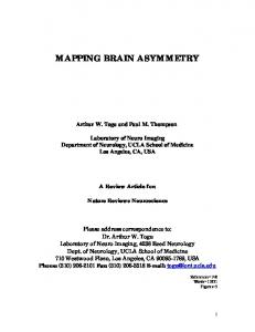
Figure 2. Typical MEG and EEG equipment. Top left: An elastic EEG cap with 60 electrodes. Top right: An MEG system, which can be operated both in seated upright (bottom left) and supine horizontal (bottom right) positions. EEG recordings can be performed concurrently with the MEG's, using magnetically-compatible electrodes and wires. Illustrations adapted courtesy of Elekta.

liters of liquid helium are necessary on a weekly basis to keep the system up to performance. Liquid nitrogen is not considered as an alternative because of the relatively higher thermal noise levels it would allow in the circuitry of current detectors. Ancillary refrigeration e.g., using liquid nitrogen just like in MR systems is not an option either, for the main reason that MEG sensors need to be located as close to the head as possible. Hence interleaving another container between the helium-cooled sensors and the subject would increase the distance between the sources and the measurement locations, therefore decreasing SNR. Some MEG sites currently experiment solutions to recycle some of the helium that naturally boils o from the MEG gantry. This approach is optimal if gas liquefaction equipment is available in the proximity of the MEG site. Under the best circumstances, this technique allows the recuperation and re-utilization of about 60% to 90% of the original helium volume. Thermal insulation is obviously a challenge in terms of safety of the subject, limited boil-o rate and minimal distance to neural sources. The technology involved uses thin sheets of berglass separated with vacuum, which brings the pick-up coils only a couple of centimeters away from the head surface, with total comfort to the subject. The MEG instrument therefore consists of a rigid helmet containing the sensors, supplemented by a reservoir of liquid helium. Though the MEG equipment is obviously not ambulatory, most commercial systems can operate with subjects in seated (upright) and horizontal (supine) positions (Fig.

ELECTROMAGNETIC BRAIN MAPPING magnet i cf i el ds( f T)

di st ances( m)

7

r el at i vesoundpr essur el evel s

Gal axy MRI

Sol arsyst em Ear t hst at i cf i el d St ungr enades

Tr af f i c

Hear t

Count r y

Tr af f i cnoi se@ 10m

Muscl es/Eyebl i nks MEG

Jetengi ne@ 100m

Cour tyar d

Nor malt al ki ng@ 1m Cal mr oom Audi t or yt hr eshol d

Figure 3. Scales of magnetic elds in a typical MEG environment (in femto- Tesla), compared to equivalent distance measures (in meters) and relative sound pressure levels. A MEG instrument probe therefore deals with a range of environmental magnetic elds of about 10 to 12 orders of magnitude, most of which consist of nuisances and perturbations masking the brain activity.

2). Having these options is usually well-appreciated by investigators in terms of alternatives for stimulus presentation, subject comfort, etc. Working with ultra-sensitive sensors is problematic though as these latter are very good at picking up all sorts of nuisances and electromagnetic perturbations generated by external sources. The magnetically-shielded room (MSR) has been an early major improvement to MEG sensing technology. All sites in urban areas contain the MEG equipment inside the walls of an MSR, which is built from a variety of metallic alloys. Most metals are successful at capturing radio-frequency perturbations. Mu-metal (a nickel-iron alloy) is one particular material of choice: its high magnetic permeability makes it very eective at screening external static or low-frequency magnetic elds. The attenuation of electromagnetic perturbations through the MSR walls is colossal and makes MEG recordings possible, even in noisy environments like hospitals (even near MRI suites) and in the vicinity of road trac. Stimulus presentation in the MSR, especially when it requires external devices, needs to be considered carefully to avoid introducing supplementary electromagnetic perturbations. Fortunately, MEG centers can benet from most of the equipment available to fMRI studies, as it is specied along the same constraints regarding magnetic compatibility. Therefore, audio and video presentations can be performed using electrostatic transducers and beams of videoprojection. Electrical stimulation for somatosensory mapping generates artifacts of short durations that do not overlap with the earliest brain responses (>20ms latency). They can be advantageously replaced by air pus delivery. As timing is critical in MEG (and EEG), all stimulation solutions need to be driven through a computer with well-characterized timing features. For instance, some electrostatic transducers eventually conduct sound through air tubes, thereby with delays in the tens of milliseconds range that need to be properly characterized. Refresh rates of video presentation


8

need to be as short as possible to ensure quasi-immediate display. The technology involved in MEG sensing, the weekly helium rells, and the materials building the MSR, make MEG a costly piece of equipment. Exciting recent developments however contribute to constant progress in cost-eectiveness, practicality and the future of MEG sensing science. Active shielding solutions for instance are available commercially. They consist in picking-up the external magnetic elds from outside the MSR and compensate for their contribution to MEG sensors in real time. The immediate benet is in MSRs of reduced size and weight and in consequence, price. The depletion of the global stock of helium is a well-documented fact that concerns multiple technology elds, beyond MEG (MRI refrigeration, space rocket propulsion, state-of-the-art video and TV displays and yes, party balloons among others). The immediate consequence of this looming shortage is a steady price increase, hence growing operational costs for MEG. Though alternative helium resources may well not be exploited as of today, the future of biomagnetism is certainly in alternative sensing technologies. High-temperature magnetometers are being developed and are based on radically-dierent principles than the low-temperature physics of current MEG systems (Savukov & Romalis, 2005; Pannetier-Lecoeur et al., 2009). SNR and sensitivity to the lower frequency range of the electromagnetic spectrum have long been issues with these emerging technologies, which were primarily designed for nuclear magnetic resonance measurements. It appears they now have considerably matured and are ready for MEG prototyping at a larger scale. Today's MEG commercial systems are organized in whole-head sensor arrays arranged in a rigid helmet covering most of the head surface but the face area. MEG signals are recorded from about 300 channels, which sometimes consist of pairs of magnetometers to form physical gradiometers (Hämäläinen, Hari, Ilmoniemi, Knuutila, & Lounasmaa, 1993). These latter are less sensitive to far-eld sources, which are supposed to originate from distant generators (e.g., road trac, elevators, heartbeats). An important benet of MEG systems is the possibility to record EEG from dense arrays of electrodes (>60) simultaneously, thereby completing the electromagnetic signature of neural currents. Additional analog channels are usually available for miscellaneous recordings (heart monitoring (ECG), muscle activity (EMG), eye movements (EOG), respiration, skin conductance, subject's responses, etc.). Sampling rate can reach√up to 5KHz on all channels with a typical instru−15 mental noise level limited to a few fT/ Hz . One femto-Tesla (1fT) is √ 10 T. Ongoing brain signals measured with MEG are on the range of about 1050 fT/ Hz (Fig. 3), with a relatively rapid decay in amplitude as frequency increases. MEG has substantial benets with respect to EEG: 1) while EEG is strongly degraded by the heterogeneity in conductivity within head tissues (e.g., insulating skull vs. conducting scalp), this eect is extremely limited in MEG, resulting in greater spatial discrimination of neural contributions. This has important implications for source modeling as we shall see below; 2) Subject preparation time is reduced considerably; 3) Measures are absolute, i.e. they are not dependent on the choice of a reference; 4) Subject's comfort is improved as there is no direct contact of the sensors on the skin. Installation of new MEG systems is presently steadily growing within research and clinical centers (about 200 worldwide). MEG/EEG experiments can be run with the subjects in supine or seated positions. A caveat however concerns EEG recording in supine position, which may rapidly lead to


9

Figure 4. On the benets of a larger number of sensors: (a) 3D rendering of a subject's scalp surface with crosshair markers representing the locations of 151 axial gradiometers as MEG sensors (coil locations are from the VSM MedTech 151 Omega System). (b) Interpolated eld topography onto the scalp surface 50 ms following the electric stimulation of the right index nger. The elds reveal a strong and focal dipolar structure above the contralateral central cortex. (c) The number of channels has been evenly reduced to 27. Though the dipolar pattern is still detected, its spatial extension is more smeared hence the intrinsic spatial resolution of the measurements has been degraded due to the eect of interpolation between sensors, which are now quite distant from the maxima of the evoked magnetic eld pattern.

subject discomfort because occipital electrodes become painful pressure points. The quiet, room-size and fairly open environment of the MSR and Faraday cages (relatively to MRI bores), make it more friendly to most subjects. Care givers may accompany subjects during the experiment. Scenarios of most typical MEG/EEG sessions

A successful MEG or EEG study is a combination of quality instrumentation, careful practical paradigm design, and well-understood preprocessing and analysis methods integrated in ecient software tools. We shall review these latter aspects in this section.

Subject preparation We have already discussed the basics of EEG preparation to ensure that contact of electrodes with skin is of quality and stable. Additional precautions should be taken for an MEG recording session as any magnetic material carried by the subject would cause major MEG artifacts. It is therefore recommended that the subject's compatibility with MEG be rapidly checked by recording and visually inspecting their spontaneous resting activity, prior to EEG preparation and proceeding any further into the experiment. Large artifacts due to metallic and magnetic parts (coins, credit cards, some dental retainers, body piercing, bra supports, etc.) or particles (make-up, hair spray, tattoos) can be readily and visually detected as they cause major low-frequency deections in MEG traces. They are usually emphasized with respiration and/or eye blinks and/or jaw movements. Some causes of artifacts may not be easily circumvented: Research volunteers may have participated in an fMRI study, sometimes months before the MEG session. Previous participation to an MRI session is likely to have caused strong, long-term magnetization of e.g., dental retainers, which generally brings the MEG session to a premature close. On site demagnetization may


10

be attempted using `degaussing' techniques usually using a conventional magnetic tape eraser, which attenuates and scrambles magnetization with limited chances of success though. Subjects are subsequently encouraged to change to wear a gown or scrubs before completing their preparation. If EEG is recorded with MEG, electrode preparation should follow the conventional principles of good EEG practice. Additional leads for EOG, ECG, EMG may then be positioned. In state-of-the-art MEG systems, head-positioning (HPI) coils are taped to the subject's head to detect its position with respect to the sensor array while recording. This is critical as, though head motion is not encouraged, it is very likely to occur within and in between runs, especially with young children and some patients. The HPIs drive a current at some higher (∼ 300Hz) frequency that is readily detected by the MEG sensors at the beginning of each run. Each of the HPI coil can then be localized within seconds with millimeter accuracy. Some MEG systems feature the possibility for continuous head-position monitoring during the very recording and o-line head movement compensation (Wehner, Hämäläinen, Mody, & Ahlfors, 2008). Head-positioning is made possible after the locations of the HPI coils are digitized prior to sitting the subject under the MEG array (Fig. 5). The distance between HPI pairs is then checked for consistency and independently by the MEG system, which is a fundamental step in the quality control of the recordings. Noisy sensors or environment and badly secured HPI taping are sources of discrepancies between the moment of subject preparation and the actual MEG recordings and should be attended. If advanced source analysis is required, additional 3D digitization of anatomical ducial points is necessary to ensure that subsequent registration to the subject's MRI anatomical volume is successful and accurate (see below). A minimum of 3 ducial points should be localized: they usually sit by the nasion and left and right peri-auricular points (Fig. 5). To reduce ambiguity in the detection of these points in the MR volume data, they can be marked using vitamin E pills or any other solid marker that is readily visible in T1-weighted MR images, if MRI is scheduled right after the MEG session. Digitization of EEG electrode locations is also mandatory for accurate, subsequent source analysis. Overall, about 15 minutes are required for subject preparation for an MEG-only session, which can extend up to about 45 minutes if simultaneous high-density EEG is required.

Paradigm design The time dimension accessible to MEG/EEG oers some considerable variety in the design of experimental paradigms for testing virtually any basic neuroscience hypothesis. Managing this new dimension is sometimes puzzling for investigators with an fMRI neuroimaging background as MEG/EEG allows to manipulate experimental parameters and presentations in the real time of the brain, not at the much slower pace of hemodynamic responses. In a nutshell, MEG/EEG experimental design is conditioned on the type of brain responses of foremost interest to the investigator: evoked, induced or sustained. The most common experimental design by far is the interleaved presentation of transient stimuli representing multiple conditions to be tested. In this design, stimuli of various categories and valences (pictures, sounds, somatosensory electric pulses or air pus, or their combination, etc.) are presented in sequence with various inter stimulus interval (ISI) durations. ISIs are


11

Headpos i t i oni ng c oi l #1

nas i on f i duc i al

Lef tper i aur i c ul ar f i duc i al

Headpos i t i oni ng c oi l #2

(a)

(b)

HPI 2

NAS LPA

(c) Figure 5. Multimodal MEG/MRI geometrical registration. (a) 3 to 5 head-positioning indicators (HPI) are taped onto the subject's scalp. Their positions, together with 3 additional anatomical ducials (nasion, left and right peri-auricular points (NAS, LPA and RPA, respectively)) are digitized using a magnetic pen digitizer. (b) The anatomical ducials need to be detected and marked in the subject's anatomical MRI volume data: they are shown as white dots in this gure, together with 3 optional, additional points dening the anterior and posterior commissures and the interhemispheric space, for the denition of Talairach coordinates. (c) These anatomical landmarks henceforth dene a geometrical referential in which the MEG sensor locations and the surface envelopes of the head tissues (e.g., the scalp and brain surface, segmented from the MRI volume) are co-registered. MEG sensors are shown as squares positioned about the head. The anatomical ducials and HPI locations are marked using dark dots.

typically much shorter than in fMRI paradigms and range from a few tens of milliseconds to a few seconds. The benet of the high temporal resolution of MEG/EEG is twofold in that respect: 1) it allows to detect and categorize the chronometry of eects occurring after stimulus presentation (evoked or induced brain responses), and 2) it provides leverage to the investigator to manipulate the timing of stimulus presentation to emphasize the very dynamics of brain processes. The rst category of experimental designs is the most typical and has a long history of scientic investigations in the characterization of the specicity of certain brain responses to certain stimulus categories (sounds, faces, words, novelty detection, etc.) as we shall discuss in greater details below. The second category of designs aims at pushing the limits of the dynamics of brain processes: a typical situation would consist in better understanding how brain processes unfold and


12

may be conditional to a hierarchy of sequences in the treatment of stimulus information from e.g., primary sensory areas to its cognitive evaluation. This may be well exemplied by paradigms such as oddball rapid serial visual presentation (RSVP, (Kranczioch, Debener, Herrmann, & Engel, 2006) and see Fig. 6), or when investigating time-related eects such as the attentional blink (Sergent, Baillet, & Dehaene, 2005; Dux & Marois, 2009). Steady-state brain responses triggered by sustained stimulus presentations belong also to this category. Here, a stimulus with specic temporal encoding (e.g., visual pattern reversals or sound modulations at a well-dened frequency) is presented and may trigger brain responses locked to the stimulus presentation rate or some harmonics. This approach is sometimes called `frequency-tagging' (of brain responses). This has led to a rich literature of steady-state brain responses in the study of multiple brain systems (Ding, Sperling, & Srinivasan, 2006; Bohórquez & Ozdamar, 2008; Parkkonen, Andersson, Hämäläinen, & Hari, 2008; Vialatte, Maurice, Dauwels, & Cichocki, 2009) and new strategies for brain computer interfaces (see e.g., (Mukesh, Jaganathan, & Reddy, 2006)). As a benecial rule of thumb for stimulus presentation in MEG/EEG paradigms, it is important to randomize the ISI durations as much as possible for most paradigms, to minimize the eect of stimulus occurrence expectancy from the subjects. Indeed, this latter triggers brain activity patterns that have been well characterized in multiple EEG studies (Clementz, Barber, & Dzau, 2002; Mnatsakanian & Tarkka, 2002) and which may bias both the subsequent MEG/EEG and behavioral responses (e.g., reaction times) to stimulation.

Data acquisition A typical MEG/EEG session consists of usually several runs. A run is a series of experimental trials. A trial is an experimental event whereby a stimulus has been presented to a subject, or the subject has performed a predened action, within a certain condition of the paradigm. Trials and runs certainly vary in duration and length depending on experimental contingencies, but it is certainly a good advice to try to keep these numbers relatively low. It is most benecial to the subject's comfort and vigilance to keep the duration of a run under 10 minutes, and preferably 5 minutes. Longer runs augment the participant's fatigue, which most commonly results in more frequent eye blinks, head movements and poorer compliance to the task instructions. For the same reasons, it is not recommended that a full session lasts longer than about 2 hours. Communication with the subject is made possible at all times via two-way intercom and video monitoring. Setting the data sampling rate is the rst parameter to decide upon when starting an MEG/EEG acquisition. Most recent systems can reach up to 5KHz per channel, which is certainly doable but leads to large data les that may be cumbersome to manipulate o-line. The sampling rate parameter is critical as it conditions the span of the frequency spectrum of the data. Indeed, this latter is limited in theory to half the sampling rate, while good practice would rather consider it is limited to about one third of the sampling frequency. As we shall see below, a vast majority of studies target brain responses that are evoked by stimulation and revealed after trial averaging. Most of these responses have a typical halfcycle of about 20ms and above, hence a characteristic frequency of 100Hz. A sampling rate of 300 to 600Hz would therefore be a safe choice. As briey discussed above, high-frequency oscillatory responses in the brain have however been evidenced in the somatosensory cortex and may reach up to about 900Hz (Cimatti et al., 2007). They therefore necessitate higher


13

t ar get

Figure 6. A typical event-related paradigm design for MEG/EEG. The experiment consists of the detection of a visual òddball'. Pictures of faces are presented very rapidly to the participants every 100ms, for a duration of 50ms and an ISI of 50ms. In about 15% of the trials, a face known to the participant is presented. This is the target stimulus and the participant needs to count the number of times he/she has seen the target individual among the unknown, distracting faces. Here, the experiment consisted of 4 runs of about 200 trials, hence resulting in a total of 120 target presentations. Typical surface data and source imaging for this paradigm are displayed in Figs. 8 and 13, respectively.

sampling rates of about 3 to 5KHz. Storage and le handling issues may arise though, as every minute of recording corresponds to about 75MB of data, sampled at 1KHz on 300 MEG and 60 EEG channels. During acquisition, MEG and EEG operators shall proceed to basic quality controls of the recordings. So called `bad channels' may be readily detected because of evident larger noise amounts in the traces, and shall be addressed (by e.g., posing more gel under the electrode or tuning the decient MEG channel). Filters may be applied during the recording, though only with caution. Indeed, bandpass lters for display only are innocuous to subsequent analysis, but most MEG/EEG instruments feature lters that are applied denitely to the actual data being recorded. The investigator shall be well aware of these parameters, which may transform into roadblocks to the analysis of some components of interest in the signals. A typical example is a low-pass lter applied at 40Hz, which prohibits subsequent access to any upper frequency ranges. Notch lters are usually applied during acquisition to attenuate power line contamination at 50 or 60Hz, though without preventing possible nuisances at some harmonics. Low-pass


14

anti-aliasing lters are generally applied by default during acquisition before analog-to digital conversion of signals and their cuto frequency is conditioned to the data sampling rate: it is conventionally set to about a third of the sampling frequency. As a general recommendation, it is suggested to keep ltering to the minimum required during acquisition i.e. anti-aliasing and optionally, a high-pass lter set at about 0.3Hz to attenuate slow DC drifts, if of no interest to the experiment because much can be performed o-line during the pre-processing steps of signal analysis, which we shall review now. Data pre-processing

The frequency spectrum of MEG/EEG data is rich and complex. Multiple processes take place simultaneously and engage neural populations at various spatial, temporal and frequency scales (Varela et al., 2001). The purpose of data pre-processing is to enhance the levels of signals of interest, while attenuating nuisances or even rejecting some episodes in the recordings that are tarnished by artifacts. In the following subsections, it is presupposed that the investigator is able to specify even at a crude level of details the basic temporal and frequency properties of the signals of interest carrying the eects being tested in the experiment. In a nutshell, it is important to target upfront, a well-dened range of brain dynamics in the course of the design of the paradigm and of the analysis pipeline.

Digital ltering As briey discussed above, data ltering is a conceptually simple, though powerful technique to extract signals within a predened frequency band of interest. This o-line data pre-processing step is the realm of digital ltering: an important and sophisticated subeld of electrical engineering (Hamming, 1983). Applying a lter to the data presupposes that the information carried by signals will be mostly preserved, to the benet of attenuating other frequency components of supposedly, no interest. Not every digital lter is suitable to the analysis of MEG/EEG traces. Indeed, the performances of lters are dened from basic characteristics such as the attenuation outside the bandpass of the frequency response, stability, computational eciency and most importantly, the introduction of phase delays. This latter is a systematic by-product of ltering and some lters may be particularly inappropriate in that respect: innite impulse response (IIR) digital lters are usually more computationally ecient than nite impulse response (FIR) alternatives, but with the inconvenient of introducing non-linear frequency-dependent phase delays; hence some non-equal delays in the temporal domain at all frequencies, which is unacceptable for MEG/EEG signal analysis where timing and phase measurements are crucial. FIR lters delay signals in the time domain equally at all frequencies, which can be conveniently compensated for by applying the lter twice: once forward and once backward on the MEG/EEG time series (Oppenheim, Schafer, & Buck, 1999). Note however some possible edge eects of the FIR lter at the beginning and end of the time series, and the necessity of a large number of time samples when applying lters with low high-pass cuto frequencies (as the length of the lter's FIR increases). Hence it is generally advisable to apply digital high-pass lters on longer episodes of data, such as on the original `raw' recordings, before these latter are chopped into epochs of shorter durations about each trial for further analysis.


15

Figure 7. Digital band-pass ltering applied to spontaneous MEG data during an interictal epileptic spike event (total epoch of 700ms duration, sampled at 1KHz). The time series of 306 MEG sensors are displayed using a buttery plot, whereby all waveforms are overlaid within the same axes. The top row displays the original data with digital lters applied during acquisition between 1.5 and 330Hz. The bottom row is a pre-processed version of the same data, band-passed ltered between 2 and 30Hz. Note how this version of the data better reveals the epileptic event occurring about time t=0ms. The corresponding sensor topographies of MEG measures are displayed to the right. The gray scale display represents the intensity of the magnetic eld captured at each sensor location and interpolated over a attened version of the MEG array (nose pointing upwards). Note also how digital band-pass ltering strongly alters the surface topography of the data, by revealing a simpler dipolar pattern over the left temporo-occipital areas of the array.

Bringing more details to the discussion would reach outside the scope of this book. The investigator should nevertheless be well aware of the potential pitfalls of analysis techniques in general, and of digital lters in particular. Although commercial software tools are well equipped with adequate lter functions, in-house or academic software solutions should be rst evaluated with great caution.

Advanced data correction techniques Despite all the precautions to obtain clean signals from EEG and MEG sensors, electrophysiological traces are likely to be contaminated by a wide variety of artifacts. These include other sources than the brain and primarily the eyes, the heart, muscles (head or limb motion, muscular tension due to postural discomfort or fatigue), electromagnetic perturbations from other devices used in the experiment and leaking power line contamination, etc. The key challenge is that most of these factors of nuisance contribute to MEG/EEG recordings with signicantly more power than ongoing brain signals (a factor of about 50 for heartbeats, eye-blinks and movements, see Fig.3). Whether experimental trials contaminated by artifacts need to be discarded requires that these latter be properly detected in the rst place. The literature of methods for tackling noise detection, attenuation and correction is too


16

immense to be properly covered in this chapter. In a nutshell, the chances of detecting and correcting artifacts are higher when these latter are monitored by a dedicated measurement. Hence electrophysiological monitoring (ECG, EOG, EMG, etc.) is strongly encouraged in most experimental settings. Some MEG solutions use additional magnetic sensors located away from the subject's head to capture the environmental magnetic elds inside the MSR. Adaptive ltering techniques may then be applied quite eectively (Haykin, 1996). The resulting additional recordings may also be used as artifact templates for visual or automatic inspection of the MEG/EEG data. For steady-state perturbations, which are thought to be independent of the brain processes of interest, empirical statistics obtained from a series of representative events (e.g., eye-blinks, heartbeats) are likely to properly capture the nuisance they systematically generate in the MEG/EEG recordings. Approaches like principal or independent component analysis (PCA and ICA, respectively) have proven to be eective in that respect for both conventional MEG/EEG and simultaneous EEG/fMRI recordings (Nolte & Hämäläinen, 2001; Pérez, Guijarro, & Barcia, 2005; Delorme, Sejnowski, & Makeig, 2007; Koskinen & Vartiainen, 2009). Modality-specic noise attenuation techniques, like signal space separation and alike (SSS), have been proposed for MEG (Taulu, Kajola, & Simola, 2004). They basically consist in designing software spatial lters that attenuate sources of nuisance that originate from outside a virtual spherical volume designed to contain the subject's head within the MEG helmet. Ultimately, the decision whether episodes contaminated by well-identied artifacts need to be discarded or corrected belongs to the investigator. Some scientists design their paradigms so that the number of trials is large enough that a few may be discarded without putting the analysis to jeopardy.

Epoch averaging: evoked responses across trials An enduring tradition of MEG/EEG signal analysis consists in enhancing brain responses that are evoked by a stimulus or an action, by averaging the data about each event dened as an epoch across trials. The underlying assumption is that there exist some consistent brain responses that are time-locked and so-called 'phase-locked' to a specic event (again e.g., the presentation of a stimulus or a motor action). Hence, it is straightforward to enhance these responses by proceeding to epoch averaging across trials, under the assumption that the rest of the data is inconsistent in time or phase with respect to the event of interest. This simple practice has permitted a vast amount of contributions to the eld of event-related potentials (in EEG, ERP) and elds (in MEG, ERF) (Handy, 2004; Niedermeyer & Silva, 2004). Trial averaging necessitates that epochs be dened about each event of interest (e.g. the stimulus onset, or the subject's response, etc.). An epoch has a certain duration, usually dened with respect to the event of interest (pre and post-event). Averaging epochs across trials can be conducted for each experimental condition at the individual and the group levels. This latter practice is called `grand-averaging' and has been made possible originally because electrodes are positioned on the subject's scalp according to montages, which are dened with respect to basic, reproducible geometrical measures taken on the head. The international 10-20 system was developed as a standardized electrode positioning and naming nomenclature to allow direct comparison of studies across the EEG community (Niedermeyer & Silva, 2004). Standardization of sensor placement does not exist in the MEG community,


17

as the sensor arrays are specic to the device being used and subject heads t dierently under the MEG helmet. Therefore, grand or even inter-run averaging is not encouraged in MEG at the sensor level without applying movement compensation techniques, or without at least checking that limited head displacements occurred between runs. Note however that trial averaging may be performed on the source times series of the MEG or EEG generators. In this latter situation, typical geometrical normalization techniques such as those used in fMRI studies need to be applied across subjects and are now a more consistent part of the MEG/EEG analysis pipeline. Once proper averaging has been completed, measures can be taken on ERP/ERF components. Components are dened as waveform elements that emerge from the baseline of the recordings. They may be characterized in terms of e.g., relative latency, topography, amplitude and duration with respect to baseline or a specic test condition. Once again, the ERP/ERF literature is immense and cannot be summarized in these lines. Multiple reviews and textbooks are available and describe in great details the specicity and sensitivity of event-related components. In the context of Social Neuroscience, let us just cite some recent MEG and EEG studies concerning: emotion face perception (Vuilleumier & Pourtois, 2007), gaze (George & Conty, 2008; Holmes, Mogg, Garcia, & Bradley, 2010), visual induction of emotions (Rudrauf et al., 2009) and imitation tasks (Biermann-Ruben et al., 2008), among many others. Phase-locked ERP/ERF components capture only the part of task-related brain responses that repeat consistently in latency and phase with respect to an event. One might however question the physiological origins and relevance of such components in the framework of oscillatory cell assemblies, as a possible mechanism ruling most basic electrophysiological processes (Gray, König, Engel, & Singer, 1989; Silva, 1991; David & Friston, 2003; Vogels, Rajan, & Abbott, 2005). This has led to a fair amount of controversy, whereby evoked components would rather be considered as artifacts of event-related, induced phase resetting of ongoing brain rhythms, mostly in the alpha frequency range ([8,12]Hz) (Makeig et al., 2002). Under this assumption, epoch averaging would only provide a secondary and poorly specic window on brain processes: this is is certainly quite severe. Indeed, event-related amplitude modulations hence not phase eects of ongoing alpha rhythms have been reported as major contributors to the slower event-related components captured by ERP/ERF's (Mazaheri & Jensen, 2008). Some authors associate these modulations of event-related amplitudes to local enhancements/reductions of event-related synchronization/desynchronization (ERS/ERD) within cell assemblies. The underlying assumption is that as the activity of more cells tends to be synchronized, the net ensemble activity will build up to an increase in signal amplitude (Pfurtscheller & Silva, 1999).

Epoch averaging: induced responses across trials Massive event-related cell synchronization is not guaranteed to take place with consistent temporal phase with respect to the onset of the event. It is therefore relatively easy to imagine that averaging trials when such phase jitters occurs across event repetitions would lead to decreased eect sensitivity. This assumption can be further elaborated in the theoretical and experimental framework of distributed, synchronized cell assemblies during perception and cognition (Varela et al., 2001; Tallon-Baudry, 2009). The seminal works by Gray and Singer in cat vision have shown that synchronization of oscillatory responses


+120ms

18

+131ms

+164ms

+204ms

+248ms

+300ms

Figure 8. Event-related, evoked MEG surface data in a visual oddball RSVP paradigm (Fig. 6). The data was interpolated between sensors and projected on a attened version of the MEG channel array. Shades of gray represent the inward and outward magnetic elds picked-up outside the head during the [120, 300] ms time interval following the presentation of the target face object. The spatial distribution of magnetic elds over the sensor array is usually relatively smooth and reveals some characteristic shape patterns that indicate that brain activity is rapidly changing and propagating during the time window. A much clearer insight can be provided by source imaging, as illustrated Fig. 13.

of spatially distributed cell ensembles is a way to establish relations between features in dierent parts of the visual eld (Gray et al., 1989). These authors evidenced that these phenomena take place in the gamma range ([40,60]Hz) i.e., a upper frequency range of the event-elated responses. These results have been conrmed by a large number of subsequent studies in animals and implanted electrodes in humans, which all demonstrated that these event-related responses could only be captured with an approach to epoch averaging that would be robust to phase jitters across trials (Tallon-Baudry, Bertrand, Delpuech, & Permier, 1997; Rodriguez et al., 1999). More evidence of gamma-range brain responses detected with EEG and MEG scalp techniques are being reported as analysis techniques are being rened and distributed to a greater community of investigators (Hoogenboom, Schoelen, Oostenveld, Parkes, & Fries, 2006). It is striking to note that as a greater number of investigations are conducted, the frequency range of gamma responses of interest is constantly expanding and now reaches between [30,100]Hz and above. As a caveat, this frequency range is also most favorable to contamination from muscle activity, such as phasic contractions or micro-saccades, which may also happen to be task-related (Yuval-Greenberg & Deouell, 2009; Melloni, Schwiedrzik,


19

Wibral, Rodriguez, & Singer, 2009). Therefore great precautions must be brought to rule out possible confounds in that matter. An additional interesting feature of gamma responses for neuroimagers is that there is a growing body of evidence showing that they tend to be more specically coupled to the hemodynamics responses captured in fMRI than other components of the electrophysiological responses (Niessing et al., 2005; Lachaux et al., 2007; Koch, Werner, Steinbrink, Fries, & Obrig, 2009). Because induced responses are mostly characterized by phase jitters across trials, averaging MEG/EEG traces in the time domain would be detrimental to the extraction of induced signals from the ongoing brain activity (David & Friston, 2003). A typical approach to the detection of induced components once again builds on the hypothesis of systematic emission of event-related oscillatory bursts limited in time duration and frequency range. Time-frequency decomposition (TFD) is a methodology of choice in that respect, as it proceeds to the estimation of instantaneous power in the time-frequency domain of time series. TFD is insensitive to variations of the signal phase when computing the average signal power across trials. TFD is a very active eld of signal processing and one of the core tools for TFD is wavelet signal decomposition. Wavelets feature the possibility to perform the spectral analysis of non-stationary signals, which spectral properties and contents are evolving with time (Mallat, 1998). This is typical of phasic electrophysiological responses for which Fourier spectral analysis is not adequate because it is based on signal stationarity assumptions (Kay, 1988). Hence, even though the typical statistics of induced MEG/EEG signal analysis is the trial mean (i.e. sample average), it is performed with a dierent measure: the estimation of short-term signal power, decomposed in time and frequency bins. Several academic and commercial software solutions are now available to perform such analysis (and the associated inference statistics) on electrophysiological signals.

New trends and methods: connectivity/complexity analysis The analysis of brain connectivity is a rapidly evolving eld of Neuroscience, with signicant contributions from new neuroimaging techniques and methods (Bandettini, 2009). While structural and functional connectivity has been emphasized with MRI-based techniques (Johansen-Berg & Rushworth, 2009; K. Friston, 2009), the time resolution of MEG/EEG oers a unique perspective on the mechanisms of rapid neural connectivity engaging cell assemblies at multiple temporal and spatial scales. We may summarize the research taking place in that eld by mentioning two approaches that have developed somewhat distinctly in the recent years, though we might predict they will ultimately converge with forthcoming research eorts. We shall note that most of the methods summarized below are also applicable to the analysis of MEG/EEG source connectivity and are not restricted to the analysis of sensor data. We further emphasize that connectivity analysis is easily fooled by confounds in the data, such as volume conduction eects i.e., smearing of scalp MEG/EEG data due to the distance from brain sources to sensors and the conductivity properties of head tissues, as we shall discuss below which need to be carefully evaluated in the course of the analysis (Nunez et al., 1997; Marzetti, Gratta, & Nolte, 2008). The rst strategy has inherited directly from the compelling intracerebral recording


20

results demonstrating that cell synchronization is a central feature of neural communication (Gray et al., 1989). Signal analysis techniques dedicated to the estimation of signal interdependencies in the broad sense have been largely applied to MEG/EEG sensor traces. Contrarily to what is appropriate to the analysis of fMRI's slow hemodynamics, simple correlation measures in the time domain are thought not to be able to capture the specicity of electrophysiological signals, which components are dened over a fairly large frequency spectrum. Coherence measures are certainly amongst the techniques the most investigated in MEG/EEG, because they are designed to be sensitive to simultaneous variations of power that are specic to each frequency bin of the signal spectrum (Nunez et al., 1997). There is however a competitive assumption that neural signals may synchronize their phases, without the necessity of simultaneous, increased power modulation (Varela et al., 2001). Waveletbased techniques have therefore been developed to detect episodes of phase synchronization between signals (Lachaux, Rodriguez, Martinerie, & Varela, 1999; Rodriguez et al., 1999). Connectivity analysis has also been recently studied through the concept of causality, whereby some neural regions would inuence others in a non-symmetric, directed fashion (Gourévitch, Bouquin-Jeannès, & Faucon, 2006). The possibilities to investigate directed inuence between not only pairs, but larger sets of time series (i.e. MEG/EEG sensors or brain regions) are vast and are therefore usually ruled by parametric models. These latter may either be related to the denition of the time series (i.e. through auto-regressive modeling for Granger-causality assessment (Lin et al., 2009)), or to the very underlying structure of the connectivity between neural assemblies (i.e., through structural equation modeling (Astol et al., 2005) and dynamic causal modeling (David et al., 2006; Kiebel, Garrido, Moran, & Friston, 2008)). The second approach to connectivity analysis pertains to the emergence of complex networks studies and associated methodology. Complex networks science is a recent branch of applied mathematics that provides quantitative tools to identify and characterize patterns of organization among large inter-connected networks such as the Internet, air transportation systems, mobile telecommunication. In neuroscience, this strategy rather concerns the identication of global characteristics of connectivity within the full array of brain signals captured at the sensor or source levels. With this methodology, the concept of the brain connectome has recently emerged, and encompasses new challenges for integrative neurosciences and the technology, methodology and tools involved in neuroimaging, to better embrace spatially-distributed dynamical neural processes at multiple spatial and temporal scales (Sporns, Tononi, & Kötter, 2005; Deco, Jirsa, Robinson, Breakspear, & Friston, 2008). From the operational standpoint, brain `connectomics' is contributing both to theoretical and computational models of the brain as a complex system (Honey, Kötter, Breakspear, & Sporns, 2007; Izhikevich & Edelman, 2008), and experimentally, by suggesting new indices and metrics such as nodes, hubs, eciency, modularity, etc. to characterize and scale the functional organization of the healthy and diseased brain (Bassett & Bullmore, 2009). This type of approaches is very promising, and calls for large-scale validation and maturation to connect with the well-explored realm of basic electrophysiological phenomena. Electromagnetic source imaging

The quantitative analysis of MEG/EEG sensor data is a source of vast possibilities to characterize time-resolved brain activity. Some studies however may require a more direct


21

assessment of the anatomical origins of the eects detected at the sensor level. It is also likely that some eects may not even be revealed using scalp measures, because of severe mixing and smearing due to the relative large distance from sources to sensors and volume conduction eects. Electromagnetic source imaging addresses this issue by characterizing these latter elements (the head shape and size, relative position and properties of sensors, noise statistics, etc.) in a principled manner and by suggesting a model for the generators responsible for the signals in the data. Ultimately, models of electrical source activity are produced and need to be analyzed in a multitude of dimensions: amplitude maps, time/frequency properties, connectivity, etc., using statistical assessment techniques. The rest of this chapter details most of the steps required, while skipping technical details, which can be found in the references cited.

MEG/EEG source estimation as a modeling problem Forward and inverse modeling From a methodological standpoint, MEG/EEG source modeling is referred to as an ìnverse problem', an ubiquitous concept, well-known to physicists and mathematicians in a wide variety of scientic elds: from medical imaging to geophysics and particle physics (Tarantola, 2004). The inverse problem framework helps conceptualize and formalize the fact that, in experimental sciences, models are confronted to observations to draw specic scientic conclusions and/or estimate some parameters that were originally unknown. Parameters are quantities that might be changed without fundamentally violating and thereby invalidating the theoretical model. Predicting observations from a model with a given set of parameters is called solving the forward modeling problem. The reciprocal situation where observations are used to estimate the values of some model parameters is the inverse modeling problem. In the context of brain functional imaging in general, and MEG/EEG in particular, we are essentially interested in identifying the neural sources of external signals observed outside the head (non invasively). These sources are dened by their locations in the brain and their amplitude variations in time. These are the essential unknown parameters that MEG/EEG source estimation will reveal, which is a typical incarnation of an inverse modeling problem. Forward modeling in the context of MEG/EEG consists in predicting the electromagnetic elds and potentials generated by any arbitrary source model, that is, for any location, orientation and amplitude parameter values of the neural currents. In general, MEG/EEG forward modeling considers that some parameters are known and xed: the geometry of the head, conductivity of tissues, sensor locations, etc. This will be discussed in the next section. As an illustration, take a single current dipole as a model for the global activity of the brain at a specic latency of an MEG averaged evoked response. We might choose to let the dipole location, orientation and amplitude as the set of free parameters to be inferred from the sensor observations. We need to specify some parameters to solve the forward modeling problem consisting in predicting how a single current dipole generates magnetic elds on the sensor array in question. We might therefore choose to specify that the head geometry will be approximated as a single sphere, with its center at some given coordinates (see Fig. 9).

ELECTROMAGNETIC BRAIN MAPPING s c al pdat a f r om br ai nac t i v i t y

( a)

pr edi c t i onsf r om f or war d andi nv er s emodel s

( b)

22 r es i dual s : dat al ef tunex pl ai ned bymodel s

( c )

Figure 9. Modeling illustrated: (a) Some unknown brain activity generates variations of magnetic elds and electric potentials at the surface of the scalp. This is illustrated by time series representing measurements at each sensor lead. (b) Modeling of the sources and of the physics of MEG and EEG. As naively represented here, forward modeling consists of a simplication of the complex geometry and electromagnetic properties of head tissues. Source models are presented with colored arrow heads. Their free parameters e.g., location, orientation and amplitude are adjusted during the inverse modeling procedure to optimize some quantitative index. This is illustrated here in (c), where the residuals i.e., the absolute dierence between the original data and the measures predicted by a source model are minimized.

A fundamental principle is that, whereas the forward problem has a unique solution in classical physics (as dictated by the causality principle), the inverse problem might accept multiple solutions, which are models that equivalently predict the observations. In MEG and EEG, the situation is critical: It has been demonstrated theoretically by von Helmoltz back in the XIXth century that the general inverse problem that consists in nding the sources of electromagnetic elds outside a volume conductor has an innite number of solutions. This issue of non-uniqueness is not specic to MEG/EEG: geophysicists for instance are also confronted to non-uniqueness in trying to determine the distribution of mass inside a planet by measuring its external gravity eld the globe. Hence theoretically, an innite number of source models equivalently ts any MEG and EEG observations, which would make them poor techniques for scientic investigations. Fortunately, this question has been addressed with the mathematics of ill-posedness and inverse modeling, which formalize the necessity of bringing additional contextual information to complement a basic theoretical model. Hence the inverse problem is a true modeling problem. This has both philosophical and technical impacts on approaching the general theory and the practice of inverse problems (Tarantola, 2004). For instance, it will be important to obtain measures of uncertainty on the estimated values of the model parameters. Indeed, we want to avoid situations where a


23

large set of values for some of the parameters produce models that equivalently account for the experimental observations. If such situation arises, it is important to be able to question the quality of the experimental data and maybe, falsify the theoretical model.

Ill-posed inverse problems. The non-uniqueness of the solution is a situation where an inverse problem is said to be ill-posed. In the reciprocal situation where there is no value for the system's parameters to account for the observations, the data are said to be inconsistent (with the model). Another critical situation of ill-posedness is when the model parameters do not depend continuously on the data. This means that even tiny changes on the observations (e.g., by adding a small amount of noise) trigger major variations in the estimated values of the model parameters. This is critical to any experimental situations, and in MEG/EEG in particular, where estimated brain source amplitudes are sought not to `jump' dramatically from millisecond to millisecond. The epistemology and early mathematics of ill-posedness have been paved by Jacques Hadamard in (Hadamard, 1902), where he somehow radically stated that problems that are not uniquely solvable are of no interest whatsoever. This statement is obviously unfair to important questions in science such as gravitometry, the backwards heat equation and surely MEG/EEG source modeling. The modern view on the mathematical treatment of ill-posed problems has been initiated in the 1960's by Andrei N. Tikhonov and the introduction of the concept of regularization, which spectacularly formalized a Solution of ill-posed problems (Tikhonov & Arsenin, 1977). Tikhonov suggested that some mathematical manipulations on the expression of ill-posed problems could make them turn well-posed in the sense that a solution would exist and possibly be unique. More recently, this approach found a more general and intuitive framework using the theory of probability, which naturally refers to the uncertainty and contextual a priori inherent to experimental sciences (see e.g., (Tarantola, 2004)). As of 2010, more than 2000 journal articles referred in the U.S. National Library of Medicine publication database to the query `(MEG OR EEG) AND source'. This abundant literature may be considered ironically as only a small sample of the innite number of solutions to the problem, but it is rather a reection of the many dierent ways MEG/EEG source modeling can be addressed by considering additional information of various nature. Such a large amount of reports on a single, technical issue has certainly been detrimental to the visibility and credibility of MEG/EEG as a brain mapping technique within the larger functional brain mapping audience, where the fMRI inverse problem is reduced to the wellposed estimation of the BOLD signal (though it is subject to major detection issues). Today, it seems that a reasonable degree of technical maturity has been reached by electromagnetic brain imaging using MEG and/or EEG. All methods reduce to only a handful of classes of approaches, which are now well-identied. Methodological research in MEG/EEG source modeling is now moving from the development of inverse estimation techniques, to statistical appraisal and the identication of functional connectivity. In these respects, it is now joining the concerns shared by other functional brain imaging communities (Salmelin & Baillet, 2009). Modeling the electromagnetics of head tissues


24

Models of neural generators. MEG/EEG forward modeling requires two basic models that are bound to work together in a complementary manner: a physical model of neural sources, and a model that predicts how these sources generate electromagnetic elds outside the head. The canonical source model of the net primary intracellular currents within a neural assembly is the electric current dipole. The adequacy of a simple, equivalent current dipole (ECD) model as a building block of cortical current distributions was originally motivated by the shape of the scalp topography of MEG/EEG evoked activity observed (Fig. 8). This latter consists essentially of (multiple) so-called `dipolar distributions' of inward/outward magnetic elds and positive/negative electrical potentials. From a historical standpoint, dipole modeling applied to EEG and MEG surface data was a spin-o from the considerable research on quantitative electrocardiography, where dipolar eld patterns are also omnipresent, and where the concept of ECD was contributed as early as in the 1960s (Geselowitz, 1964). However, although cardiac electrophysiology is well captured by a simple ECD model because there is not much questioning about source localization, the temporal dynamics and spatial complexity of brain activity may be more challenging. Alternatives to the ECD model exist in terms of the compact, parametric representation of distributed source currents. They consist either of higher-order source models called multipoles (Jerbi, Mosher, Baillet, & Leahy, 2002; Jerbi et al., 2004) also derived from cardiographic research (Karp, Katila, Saarinen, Siltanen, & Varpula, 1980) or densely-distributed source models (Wang, Williamson, & Kaufman, 1992). In the latter case, a large number of ECD's are distributed in the entire brain volume or on the cortical surface, thereby forming a dense grid of elementary sites of activity, which intensity distribution is determined from the data. To understand how these elementary source models generate signals that are measurable using external sensors, further modeling is required for the geometrical and electromagnetic properties of head tissues, and the properties of the sensor array. Modeling the sensor array. The details of the sensor geometry and pick-up technology are dependent on the manufacturer of the array. We may however summarize some fundamental principles in the next following lines. We have already reviewed how the sensor locations can be measured with state-ofthe-art MEG and EEG equipment. If this information is missing, sensor locations may be roughly approximated from montage templates, but this will be detrimental to the accuracy of the source estimates (Schwartz, Poiseau, Lemoine, & Barillot, 1996). This is critical with MEG, as the subject is relatively free to position his/her head within the sensor array. Typical 10/20 EEG montages oer less degrees of freedom in that respect. Careful consideration of this geometrical registration issue using the solutions discussed above (HPI, head digitization and anatomical ducials) should provide satisfactory performances in terms of accuracy and robustness. In EEG, the geometry of electrodes is considered as point-like. Advanced electrode modeling should include the true shape of the sensor (that is, a àt' cylinder), but it is generally acknowledged that the spatial resolution of EEG measures is coarse enough to neglect this factor. One important piece of information however is the location of the reference electrode i.e., nasion, central, linked mastoids, etc. as it denes the physics of a given set of EEG measures. If this information is missing, the EEG data can be re-referenced with


25

respect to the instantaneous arithmetic average potential (Niedermeyer & Silva, 2004). In MEG, the sensing coils may also be considered point-like as a rst approximation, though some analysis software packages include the exact sensor geometry in modeling. The computation of the total magnetic ux induction captured by the MEG sensors can be more accurately modeled by the geometric integration within their surface area. Gradiometer arrangements are readily modeled by applying the arithmetic operation they mimic, combining the elds modeled at each of its magnetometers. Recent MEG systems include sophisticated online noise-attenuation techniques such as: higher-order gradient corrections and signal space projections. They contribute significantly to the basic model of data formation and therefore need to be taken into account (Nolte & Curio, 1999).

Modeling head tissues. Predicting the electromagnetic elds produced by an elemen-

tary source model at a given sensor array requires another modeling step, which concerns a large part of the MEG/EEG literature. Indeed, MEG/EEG `head modeling' studies the inuence of the head geometry and electromagnetic properties of head tissues on the magnetic elds and electrical potentials measured outside the head. Given a model of neural currents, the physics of MEG/EEG are ruled by the theory of electrodynamics (Feynman, 1964), which reduces in MEG to Maxwell's equations, and to Ohm's law in EEG, under quasistatic assumptions. These latter consider that the propagation delay of the electromagnetic waves from brain sources to the MEG/EEG sensors is negligible. The reason is the relative proximity of MEG/EEG sensors to the brain with respect to the expected frequency range of neural sources (up to 1KHz) (Hämäläinen et al., 1993). This is a very important, simplifying assumption, which has immediate consequences on the computational aspects of MEG/EEG head modeling. Indeed, the equations of electro and magnetostatics determine that there exist analytical, closed-form solutions to MEG/EEG head modeling when the head geometry is considered as spherical. Hence, the simplest, and consequently by far most popular model of head geometry in MEG/EEG consists of concentric spherical layers: with one sphere per major category of head tissue (scalp, skull, cerebrospinal uid and brain). The spherical head geometry has further attractive properties for MEG in particular. Quite remarkably indeed, spherical MEG head models are insensitive to the number of shells and their respective conductivity: a source within a single homogeneous sphere generates the same MEG elds as when located inside a multilayered set of concentric spheres with dierent conductivities. The reason for this is that conductivity only inuences the distribution of secondary, volume currents that circulate within the head volume and which are impressed by the original primary neural currents. The analytic formulation of Maxwell's equations in the spherical geometry shows that these secondary currents do not generate any magnetic eld outside the volume conductor (Sarvas, 1987). Therefore in MEG, only the location of the center of the spherical head geometry matters. The respective conductivity and radius of the spherical layers have no inuence on the measured MEG elds. This is not the case in EEG, where both the location, radii and respective conductivity of each spherical shell inuence the surface electrical potentials. This relative sensitivity to tissue conductivity values is a general, important dierence between EEG and MEG.


26

A spherical head model can be optimally adjusted to the head geometry, or restricted to regions of interest e.g., parieto-occipital regions for visual studies. Geometrical registration to MRI anatomical data improves the adjustment of the best-tting sphere geometry to an individual head. Another remarkable consequence of the spherical symmetry is that radially oriented brain currents produce no magnetic eld outside a spherically symmetric volume conductor. For this reason, MEG signals from currents generated within the gyral crest or sulcal depth are attenuated, with respect to those generated by currents owing perpendicularly to the sulcal walls. This is another important contrast between MEG and EEG's respective sensitivity to source orientation (Hillebrand & Barnes, 2002). Finally, the amplitude of magnetic elds decreases faster than electrical potentials' with the distance from the generators to the sensors. Hence it has been argued that MEG is less sensitive to mesial and subcortical brain structures than EEG. Experimental and modeling eorts have shown however that MEG can detect neural activity from deeper brain regions (Tesche, 1996; Attal et al., 2009). Though spherical head models are convenient, they are poor approximations of the human head shape, which has some inuence on the accuracy of MEG/EEG source estimation (Fuchs, Drenckhahn, Wischmann, & Wagner, 1998). More realistic head geometries have been investigated and all require solving Maxwell's equations using numerical methods. Boundary Element (BEM) and Finite Element (FEM) methods are generic numerical approaches to the resolution of continuous equations over discrete space. In MEG/EEG, geometric tessellations of the dierent envelopes forming the head tissues need to be extracted from the individual MRI volume data to yield a realistic approximation of their geometry (Fig. 10). In BEM, the conductivity of tissues is supposed to be homogeneous and isotropic within each envelope. Therefore, each tissue envelope is delimited using surface boundaries dened over a triangulation of each of the segmented envelopes obtained from MRI. FEM assumes that tissue conductivity may be anisotropic (such as the skull bone and the white matter), therefore the primary geometric element needs to be an elementary volume, such as a tetrahedron (Marin, Guerin, Baillet, Garnero, & Meunier, 1998). The main obstacle to a routine usage of BEM, and more pregnantly of FEM, is the surface or volume tessellation phase. Because the head geometry is intricate and not always well-dened from conventional MRI due to signal drop-outs and artifacts, automatic segmentation tools sometimes fail to identify some important tissue structures. The skull bone for instance, is invisible on conventional T1-weighted MRI. Some image processing techniques however can estimate the shape of the skull envelope from high-quality T1-weighted MRI data (Dogdas, Shattuck, & Leahy, 2005). However, the skull bone is a highly anisotropic structure, which is dicult to model from MRI data. Recent progress using MRI diusiontensor imaging (DTI) helps reveal the orientation of major white ber bundles, which is also a major source of conductivity anisotropy (Haueisen et al., 2002). Computation times for BEM and FEM remain extremely long (several hours on a conventional workstation), and are detrimental to rapid access to source localization following data acquisition. Both algorithmic (Huang, Mosher, & Leahy, 1999; Kybic, Clerc, Faugeras, Keriven, & Papadopoulo, 2005) and pragmatic (Ermer, Mosher, Baillet, & Leah, 2001; Darvas, Ermer, Mosher, & Leahy, 2006) solutions to this problem have however been proposed to


(a)

(b)

27

(c)

Figure 10. Three approaches to MEG/EEG head modeling: (a) Spherical approximation of the geometry of head tissues, with analytical solution to Maxwell's and Ohm's equations; (b) Tessellated surface envelopes of head tissues obtained from the segmentation of MRI data; (c) An alternative to (b) using volume meshes here built from tetrahedra. In both (b) and (c) Maxwell's and Ohm's equations need to be solved using numerical methods: BEM and FEM, respectively.

make realistic head models more operational. They are available in some academic software packages. Finally, let us close this section with an important caveat: Realistic head modeling is bound to the correct estimation of tissues conductivity values. Though solutions for impedance tomography using MRI (Tuch, Wedeen, Dale, George, & Belliveau, 2001) and EEG (Goncalves et al., 2003) have been suggested, they remain to be matured before entering the daily practice of MEG/EEG. So far, conductivity values from ex-vivo studies are conventionally integrated in most spherical and realistic head models (Geddes & Baker, 1967).

MEG/EEG source modeling For clarity purposes, we will not attempt to formalize in a general, overly technical way, the classes of approaches to MEG/EEG source estimation. We will rather adopt a pragmatic standpoint, observing that two main chapels have developed quite separately: the localization and the imaging approaches respectively (Salmelin & Baillet, 2009). Our purpose here is to mark methodological landmarks and stress on dierences, similarities, and their respective assets.

Source localization vs. source imaging. The localization approach to MEG/EEG source estimation considers that brain activity at any time instant is generated by a relatively small number (a handful, at most) of brain regions. Each source is therefore represented by an elementary model, such as an ECD, that captures local distributions of neural currents. Ultimately, each elementary source is back projected or constrained to the subject's brain volume or an MRI anatomical template, for further interpretation. In a nutshell, localization models are essentially compact, in terms of number of generators involved and their surface extension (from point-like to small cortical surface patches).


28

The alternative imaging approaches to MEG/EEG source modeling were originally inspired by the plethoric research in image restoration and reconstruction in other domains (early digital imaging, geophysics, and other biomedical imaging techniques). The resulting image source models do not yield small sets of local elementary models but rather the distribution of àll' neural currents. This results in stacks of images where brain currents are estimated wherever elementary current sources had been previously positioned. This is typically achieved using a dense grid of current dipoles over the entire brain volume or limited to the cortical gray matter surface. These dipoles are xed in location and generally, orientation, and are homologous to pixels in a digital image. The imaging procedure proceeds to the estimation of the amplitudes of all these elementary currents at once. Hence contrarily to the localization model, there is no intrinsic sense of distinct, active source regions per se. Explicit identication of activity issued from discrete brain regions usually necessitates complementary analysis, such as empirical or inference-driven amplitude thresholding, to discard elementary sources of non-signicant contribution according to the statistical appraisal. In that respect, MEG/EEG source images are very similar in essence to the activation maps obtained in fMRI, with the benet of time resolution however (see Fig. 11).

( a)

( b)

Figure 11. Inverse modeling: the localization (a) vs. imaging (b) approaches. Source modeling through localization consists in decomposing the MEG/EEG generators in a handful of elementary source contributions; the simplest source model in this situation being the equivalent current dipole (ECD). This is illustrated here from experimental data testing the somatotopic organization of primary cortical representations of hand ngers. The parameters of the single ECD have been adjusted on the [20, 40] ms time window following stimulus onset. The ECD was found to localize along the contralateral central sulcus as revealed from the 3D rendering obtained after the source location has been registered to the individual anatomy. In the imaging approach, the source model is spatially-distributed using a large number of ECD's. Here, a surface model of MEG/EEG generators was constrained to the individual brain surface extracted from T1-weighted MR images. Elemental source amplitudes are interpolated onto the cortex, which yields an image-like distribution of the amplitudes of cortical currents.

The following subsections further detail these two respective approaches.

Dipole tting: The localization approach. As discussed above, early quantitative source

localization research in electro and magnetocardiography had promoted the equivalent current dipole as a generic model of massive electrophysiological activity. Before ecient esti-


29

mation techniques and software were available, electrophysiologists would empirically solve the MEG/EEG forward and inverse problems to characterize the neural generators responsible for experimental eects detected on the scalp sensors. This approach is exemplied in (Wood, Cohen, Cun, Yarita, & Allison, 1985), where terms such as `waveform morphology' and `shape of scalp topography' are used to discuss the respective sources of MEG and EEG signals. This empirical approach to localization has considerably beneted from the constant increase in the number of sensors of MEG and EEG systems (Fig. 4). Indeed, surface interpolation techniques of sensor data have gained considerable popularity in MEG and EEG research (Perrin, Pernier, Bertrand, Giard, & Echallier, 1987): investigators now can routinely access surface representations of their data on an approximation of the scalp surface as a disc, a sphere or on the very head surface extracted from the subject's MRI. (Wood et al., 1985) like many others used the distance between the minimum and maximum magnetic distribution of the dipolar-looking eld topography to infer the putative depth of a dipolar source model of the data. Computational approaches to source localization attempt to mimic the talent of electrophysiologists, with a more quantitative benet though. We have seen that the current dipole model has been adopted as the canonical equivalent generator of the electrical activity of a brain region considered as a functional entity. Localizing a current dipole in the head implies that 6 unknown parameters be estimated from the data: 3 for location per se, 2 for orientation and 1 for amplitude. Therefore, characterizing the source model by a restricted number of parameters was considered as a possible solution to the ill-posed inverse problem and has been attractive to many MEG/EEG scientists. Without additional prior information besides the experimental data, the number of unknowns in the source estimation problem needs to be smaller than that of the instantaneous observations for the inverse problem to be well-posed, in terms of uniqueness of a solution. Therefore, recent high-density systems with about 300 sensors would theoretically allow the unambiguous identication of 50 dipolar sources; a number that would probably satisfy the modeling of brain activity in many neuroscience questions. It appears however, that most research studies using MEG/EEG source localization bear a more conservative prole, using much fewer dipole sources (typically < 5). The reasons for this are both technical and proper to MEG/EEG brain signals as we shall now discuss. Numerical approaches to the estimation of unknown source parameters are generally based on the widely-used least-squares (LS) technique which attempts to nd the set of parameter values that minimize the (square of the) dierence between observations and predictions from the model (Fig. 9). Biosignals such as MEG/EEG traces are naturally contaminated by nuisance components (e.g., environmental noise and physiological artifacts), which shall not be explained by the model of brain activity. These components however, contribute to some uncertainty on the estimation of the source model parameters. As a toy example, let us consider noise components that are independent and identically-distributed on all 300 sensors. One would theoretically need to adjust as many additional free parameters in the inverse model as the number of noise components to fully account for all possible experimental (noisy) observations. However, we would end up handling a problem with 300 additional unknowns, adding to the original 300 source parameters, with only 300 data measures available.


30

Hence, and to avoid confusion between contributions from nuisances and signals of true interest, the MEG/EEG scientist needs to determine the respective parts of interest (the signal) versus perturbation (noise) in the experimental data. The preprocessing steps we have reviewed in the earlier sections of this chapter are therefore essential to identify, attenuate or reject some of the nuisances in the data, prior to proceeding to inverse modeling. Once the data has been preprocessed, the basic LS approach to source estimation aims at minimizing the deviation of the model predictions from the data: that is, the part in the observations that are left unexplained by the source model. Let us suppose for the sake of further demonstration that the data is idealistically clean from any noisy disturbance, and that we are still willing to t 50 dipoles to 300 data points. This is in theory an ideal case where there are as many unknowns as there are instantaneous data measures. However we shall discuss that unknowns in the models do not all share the same type of dependency to the data. In the case of a dipole model, doubling the amplitude of the dipole doubles the amplitude of the sensor data. Dipole source amplitudes are therefore said to be linear parameters of the model. Dipole locations however do not depend linearly on the data: the amplitude of the sensor data is altered non-linearly with changes in depth and position of the elementary dipole source. Source orientation is a somewhat hybrid type of parameter. It is considered that small, local displacements of brain activity can be eciently modeled by a rotating dipole source at some xed location. Though source orientation is a non-linear parameter in theory, replacing a free-rotating dipole by a triplet of 3 orthogonal dipoles with xed orientations is a way to express any arbitrary source orientation by a set of 3 hence linear amplitude parameters. Non-linear parameters are more dicult to estimate in practice than linear unknowns. The optimal set of source parameters dened from the LS criterion exists and is theoretically unique when sources are constrained to be dipolar (see e.g. (Badia, 2004)). However in practice, non-linear optimization may be trapped by suboptimal values of the source parameters corresponding to a so-called local-minimum of the LS objective. Therefore the practice of multiple dipole tting is very sensitive to initial conditions e.g., the values assigned to the unknown parameters to initiate the search, and to the number of sources in the model, which increases the possibility of the optimization procedure to be trapped in local, suboptimal LS minima. In summary, even though localizing a number of elementary dipoles corresponding to the amount of instantaneous observations is theoretically well-posed, we are facing two issues that will drive us to reconsider the source-tting problem in practice: 1) The risk of overtting the data: meaning that the inverse model may account for the noise components in the observations, and 2) non-linear searches that tend to be trapped in local minima of the LS objective. A general rule of thumb when the data is noisy and the optimization principle is ruled by non-linear dependency is to keep the complexity of the estimation as low as possible. Taming complexity starts with reducing the number of unknowns so that the estimation problem becomes overdetermined. In experimental sciences, overdeterminacy is not as critical as underdeterminacy. From a pragmatic standpoint, supplementary sensors provide additional information and allow the selection of subsets of channels, which may be less contaminated by noise and artifacts. The early MEG/EEG literature is abundant in studies reporting on single dipole


31

source models. The somatotopy of primary somatosensory brain regions (Okada, Tanenbaum, Williamson, & Kaufman, 1984; Meunier, Lehéricy, Garnero, & Vidailhet, 2003), primary, tonotopic auditory (Zimmerman, Reite, & Zimmerman, 1981) and visual (Lehmann, Darcey, & Skrandies, 1982) responses are examples of such studies where the single dipole model contributed to the better temporal characterization of primary brain responses. Later components of evoked elds and potentials usually necessitate more elementary source to be tted. However, this may be detrimental to the numerical stability and signicance of the inverse model. The spatio-temporal dipole model was therefore developed to localize the sources of scalp waveforms that were assumed to be generated by multiple and overlapping brain activations (Scherg & Cramon, 1985). This spatio-temporal model and associated optimization expect that an elementary source is active for a certain duration with amplitude modulations while remaining at the same location with the same orientation. This is typical of the introduction of prior information in the MEG/EEG source estimation problem, and this will be further developed in the imaging techniques discussed below. The number of dipoles to be adjusted is also a model parameter that needs to be estimated. However it leads to dicult, and usually impractical optimization (Waldorp, Huizenga, Nehorai, Grasman, & Molenaar, 2005). Therefore the number of elementary sources in the model is often qualitatively assessed by expert users, which may question the reproducibility of such user-dependent analyses. Hence, special care should be brought to the evaluation of the stability and robustness of the estimated source models. With all that in mind, source localization techniques have proven to be eective, even on complex experimental paradigms (see e.g., (Helenius, Parviainen, Paetau, & Salmelin, 2009)). Signal classication and spatial ltering techniques are ecient alternative approaches in that respect. They have gained considerable momentum in the MEG/EEG community in the recent years. They are discussed in the following subsection.

Scanning techniques: Spatial lters, beamformers and signal classiers. The inherent

diculties to source localization with multiple generators and noisy data have led signal processors to develop alternative approaches, most notably in the glorious eld of radar and sonar in the 1970's. Rather than attempting to identify discrete sets of sources by adjusting their non-linear location parameters, scanning techniques have emerged and proceeded by systematically sifting through the brain space to evaluate how a predetermined elementary source model would t the data at every voxel of the brain volume. For this local model evaluation to be specic of the brain location being scanned, contributions from possible sources located elsewhere in the brain volume need to be blocked. Hence, these techniques are known as spatial-lters and beamformers (the simile is a virtual beam being directed and `listening' exclusively at some brain region). These techniques have triggered tremendous interest and applications in array signal processing and have percolated the MEG/EEG community at several instances (e.g., (Spencer, Leahy, Mosher, & Lewis, 1992) and more recently, (Hillebrand, Singh, Holliday, Furlong, & Barnes, 2005)). At each point of the brain grid, a narrow-band spatial lter is formed and evaluates the contribution to data from an elementary source model such as a single or a triplet of current dipoles while contributions from other brain regions are ideally muted, or at least attenuated. (Veen & Buckley, 1988) is a technical introduction to beamformers and excellent further reading.


32

It is sometimes claimed that beamformers do not solve an inverse problem: this is a bit overstated. Indeed, spatial lters do require a source and a forward model that will be both confronted to the observations. Beamformers scan the entire expected source space and systematically test the prediction of the source and forward models with respect to observations. These predictions compose a distributed score map, which should not be misinterpreted as a current density map. More technically though no details are given here the forward model needs to be inverted by the beamformer as well. It only proceeds iteratively by sifting through each source grid point and estimating the output of the corresponding spatial lter. Hence beamformers and spatial lters are truly avatars of inverse modeling. Beamforming is therefore a convenient method to translate the source localization problem into a signal detection issue. As every method that tackles a complex estimation problem, there are drawbacks to the technique: 1. Beamformers depend on the covariance statistics of the noise in the data. These latter may be estimated from the data through sample statistics. However, the number of independent data samples that are necessary for the robust and numerically stable estimation of covariance statistics is proportional to the square of the number of data channels, i.e. of sensors. Hence beamformers ideally require long, stationary episodes of data, such as sweeps of ongoing, unaveraged data and experimental conditions where behavioral stationarity ensures some form of statistical stationarity in the data (e.g., ongoing movements). (Cheyne, Bakhtazad, & Gaetz, 2006) have suggested that event-related brain responses can be well captured by beamformers using sample statistics estimated across single trials. 2. They are more sensitive to errors in the head model. The lter outputs are typically equivalent to local estimates of SNR. However this latter is not homogeneously distributed everywhere in the brain volume: MEG/EEG signals from activity in deeper brain regions or gyral generators in MEG have weaker SNR than in the rest of the brain. The consequence is side lobe leakages from interfering sources nearby, which impede lter selectivity and therefore, the specicity of source detection (Wax & Anu, 1996); 3. Beamformers may be fooled by simultaneous activations occurring in brain regions outside the lter pass-band that are highly correlated with source signals within the passband. External sources are interpreted as interferences by the beamformer, which blocks the signals of interest because they bear the same sample statistics than the interference. Signal processors had long identied these issues and consequently developed multiple signal classication (MUSIC) as an alternative technique ((Schmidt, 1986)). MUSIC assumes that signal and noise components in the data are uncorrelated. Strong theoretical results in information theory show that these components live in separate, high-dimensional data subspaces, which can be identied using e.g., a PCA of the data time series (Golub, 1996). (J. C. Mosher, Baillet, & Leahy, 1999) is an extensive review of signal classication approaches to MEG and EEG source localization. However, the practical aspects of MUSIC and its variations remain limited by their sensitivity in the accurate denition of the respective signal and noise subspaces. These techniques may be fooled by background brain activity, which signals share similar properties with the event-related responses of interest. An interesting side application of MUSIC-like powerful discrimination ability though has been developed in epilepsy spike-sorting (Ossadtchi et al., 2004).


33

In summary, spatial-lters, beamformers and signal classication approaches bring us closer to a distributed representation of the brain electrical activity. As a caveat, the results generated by these techniques are not an estimation of the current density everywhere in the brain. They represent a score map of a source model generally a current dipole that is evaluated at the points of a predened spatial lattice, which sometimes leads to misinterpretations. The localization issue now becomes a signal detection problem within the score map (J. Mosher, Baillet, & Leahy, 2003). The imaging approaches we are about to introduce now, push this detection problem further by estimating the brain current density globally.

Distributed source imaging. Source imaging approaches have developed in parallel to the techniques discussed above. Imaging source models consist of distributions of elementary sources, generally with xed locations and orientations, which amplitudes are estimated at once. MEG/EEG source images represent estimations of the global neural current intensity maps, distributed within the entire brain volume or constrained at the cortical surface. Source image supports consist of either a 3D lattice of voxels or of the nodes of the triangulation of the cortical surface. These latter may be based on a template, or preferably obtained from the subject's individual MRI and conned to a mask of the grey matter. Multiple academic software packages perform the necessary segmentation and tessellation processes from high-contrast T1-weighted MR image volumes. As discussed earlier in this chapter, the cortically-constrained image model derives from the assumption that MEG/EEG data originates essentially from large cortical assemblies of pyramidal cells, with currents generated from post-synaptic potentials owing orthogonally to the local cortical surface. This orientation constraint can either be strict (Dale & Sereno, 1993) or relaxed by authorizing some controlled deviation from the surface normal (Lin, Belliveau, Dale, & Hamalainen, 2006). In both cases, reasonable spatial sampling of the image space requires several thousands (typically ∼ 10000) of elementary sources as depicted Fig. 12. Consequently, though the imaging inverse problem consists in estimating only linear parameters, it is dramatically underdetermined. Just like in the context of source localization where e.g., the number of sources is a restrictive prior as a remedy to ill-posedness, imaging models need to be complemented by a priori information. This is properly formulated with the mathematics of regularization as we shall now briey review. Adding priors to the imaging model can be adequately formalized in the context of Bayesian inference where solutions to inverse modeling satisfy both the t to observations given some probabilistic model of the nuisances and additional priors. From a parameter estimation perspective, the maximum of the a posteriori probability distribution of source intensity, given the observations could be considered as the `best possible model'. This maximum a posteriori (MAP) estimate has been extremely successful in the digital image restoration and reconstruction communities. (Geman & Geman, 1984) is a masterpiece reference of the genre. The MAP is obtained in Bayesian statistics through the optimization of the mixture of the likelihood of the noisy data i.e., of the predictive power of a given source model with the a priori probability of a given source model. We do not want to detail the mathematics of Bayesian inference any further here as this


(a)

(b)

(c)

(d)

34

Figure 12. The cortical surface, tessellated at two resolutions, using: (a,b) 10,034 vertices (20,026 triangles with 10 mm2 average surface area) and (c,d) 79,124 vertices (158,456 triangles with 1.3 mm2 average surface area).

would reach outside the objectives of this chapter. Specic recommended further reading includes (Demoment, 1989), for a Bayesian discussion on regularization and (Baillet, Mosher, & Leahy, 2001), for an introduction to MEG/EEG imaging methods, also in the Bayesian framework. From a practical standpoint, the priors on the source image models may take multiple faces: promote current distributions with high spatial and temporal smoothness, penalize models with currents of unrealistic, non-physiologically plausible amplitudes, favor the adequation with an fMRI activation maps, or prefer source image models made of piecewise homogeneous active regions, etc. An appealing benet from well-chosen priors is that it may ensure the uniqueness of the optimal solution to the imaging inverse problem, despite its original underdeterminacy. Because relevant priors for MEG/EEG imaging models are plethoric, it is important to understand that the associated source estimation methods usually belong to the same technical background. Also, the selection of image priors can be seen as arbitrary and subjective an issue as the selection of dipoles in the source localization techniques we have reviewed previously. Comprehensive solutions for this model selection issue are now emerging and will be briey reviewed further below. The free parameters of the imaging model are the amplitudes of the elementary source


35

currents distributed on the brain's geometry. The non-linear parameters (e.g., the elementary source locations) now become xed priors as provided by anatomical information. The model estimation procedure and the very existence of a unique solution strongly depend on the mathematical nature of the image prior. A widely-used prior in the eld of image reconstruction considers that the expected source amplitudes be as small as possible on average. This is the well-described minimumnorm (MN) model. Technically speaking, we are referring to the L2-norm; the objective cost function ruling the model estimation is quadratic in the source amplitudes, with a unique analytical solution (Tarantola, 2004). The computational simplicity and uniqueness of the MN model has been very attractive in MEG/EEG early on (Wang et al., 1992). The basic MN estimate is problematic though as it tends to favor the most supercial brain regions (e.g., the gyral crowns) and underestimate contributions from deeper source areas (such as sulcal fundi) (Fuchs, Wagner, Köhler, & Wischmann, 1999). As a remedy, a slight alteration of the basic MN estimator consists in weighting each elementary source amplitude by the inverse of the norm of its contribution to sensors. Such depth weighting yields a weighted MN (WMN) estimate, which still benets from uniqueness and linearity in the observations as the basic MN (Lin, Witzel, et al., 2006). Despite their robustness to noise and simple computation, it is relevant to question the neurophysiological validity of MN priors. Indeed though reasonably intuitive there is no evidence that neural currents would systematically match the principle of minimal energy. Some authors have speculated that a more physiologically relevant prior would be that the norm of spatial derivatives (e.g., surface or volume gradient or Laplacian) of the current map be minimized (see LORETA method in (Pascual-Marqui, Michel, & Lehmann, 1994)). As a general rule of thumb however, all MN-based source imaging approaches overestimate the smoothness of the spatial distribution of neural currents. Quantitative and qualitative empirical evidence however demonstrate spatial discrimination of reasonable range at the sub-lobar brain scale (Darvas, Pantazis, Kucukaltun-Yildirim, & Leahy, 2004; Sergent et al., 2005) (Fig. 13). Most of the recent literature in regularized imaging models for MEG/EEG consists in struggling to improve the spatial resolution of the MN-based models (see (Baillet, Mosher, & Leahy, 2001) for a review) or to reduce the degree of arbitrariness involved in selected a generic source model a priori (Mattout, Phillips, Penny, Rugg, & Friston, 2006; Stephan, Penny, Daunizeau, Moran, & Friston, 2009). This results in notable improvements in theoretical performances, though with higher computational demands and practical optimization issues. As a general principle, we are facing the dilemma of knowing that all priors about the source images are certainly abusive, hence that the inverse model is approximative, while hoping it is just not too approximative. This discussion is recurrent in the general context of estimation theory and model selection as we shall discuss in the next section.

Appraisal of MEG/EEG source models Throughout this chapter, we have been dealing with modeling, and modeling implies dealing with uncertainty. MEG/EEG source estimation has uncertainty everywhere: data are complex and contaminated with various nuisances, source models are simplistic, head models have approximated geometries and conductivity properties, the choice of priors has


+120ms

36

+131ms

+164ms

+204ms

+248ms

Figure 13. Distributed source imaging of the [120, 300] ms time interval following the presentation of the target face object in the visual RSVP oddball paradigm described in Fig. 6. The images show a slightly smoothed version of one participant's cortical surface. Colors encode the contrast of MEG source amplitudes between responses to target versus control faces. Visual responses are detected by 120ms and rapidly propagate anteriorly. By 250 ms onwards, strong anterior mesial responses are detected in the cingular cortex. These latter are the main contributors of the brain response to target detection.

its share of subjectivity, etc. It is therefore reasonable to question how sensitive the numerical methods at stake are to these possible sources of errors and bias. This concerns the appraisal of the source model, which general methodology has been adapted to MEG/EEG just recently and is now achieving signicant maturity.

Condence intervals. We have discussed how tting dipoles to a data time segment may be quite sensitive to initial conditions and therefore, subjective. Similarly, imaging source models suggest that each brain location is active, potentially. It is therefore important to evaluate the condence one might acknowledge to a given model. In other words, we are now looking for error bars that would dene a condence interval about the estimated values of a source model. Signal processors have developed a principled approach to what they have coined as `detection and estimation theories' (Kay, 1993). The main objective consists in understanding how certain one can be about the estimated parameters of a model, given a model for the noise in the data. The basic approach consists in considering the estimated parameters (e.g., source locations) as distributed through random variables. Parametric estimation of


37

error bounds on the source parameters consists in estimating their bias and variance. Bias is an estimation of the distance between the true value and the expectancy of estimated parameter values due to perturbations. The denition of variance follows immediately. Cramer-Rao lower bounds (CRLB) on the estimator's variance can be explicitly computed using an analytical solution to the forward model and given a model for perturbations (e.g., with distribution under a normal law). In a nutshell, the tighter the CRLB, the more condent one can be about the estimated values. (J. C. Mosher, Spencer, Leahy, & Lewis, 1993) have investigated this approach using extensive Monte-Carlo simulations, which evidenced a resolution of a few millimeters for single dipole models. These results were later conrmed by phantom studies (Leahy, Mosher, Spencer, Huang, & Lewine, 1998; Baillet, Riera, et al., 2001). CRLB increased markedly for two-dipole models, thereby demonstrating their extreme sensitivity and instability. Recently, non-parametric approaches to the determination of error bounds have greatly beneted from the commensurable increase in computational power. Jackknife and bootstrap techniques proved to be ecient and powerful tools to estimate condence intervals on MEG/EEG source parameters, regardless of the nature of perturbations and of the source model. These techniques are all based on data resampling approaches and have proven to be exact and ecient when a large-enough number of experimental replications are available (Davison & Hinkley, 1997). This is typically the case in MEG/EEG experiments where protocols are designed on multiple trials. If we are interested e.g., in knowing about the condence interval on a source location in a single-dipole model from evoked averaged data, the bootstrap will generate a large number (typically > 500) of surrogate average datasets, by randomly choosing trials from the original set of trials and averaging them all together. Because the trial selection is random and from the complete set of trials, the corresponding sample distribution of the estimated parameter values is proven to converge toward the true distribution. A pragmatic approach to the denition of a condence interval thereby consists in identifying the interval containing e.g., 95% of the resampled estimates (see Fig. 14, (Baryshnikov, Veen, & Wakai, 2004; Darvas et al., 2005; McIntosh & Lobaugh, 2004)). These considerations naturally lead us to statistical inference, which questions hypothesis testing.

Statistical inference. Questions like: `How dierent is the dipole location between these

two experimental conditions?' and Àre source amplitudes larger in such condition that in a control condition?' belong to statistical inference from experimental data. The basic problem of interest here is hypothesis testing, which is supposed to potentially invalidate a model under investigation. Here, the model must be understood at a higher hierarchical level than when talking about e.g., an MEG/EEG source model. It is supposed to address the neuroscience question that has motivated data acquisition and the experimental design (Guilford, P., & Fruchter, B., 1978). In the context of MEG/EEG, the population samples that will support the inference are either trials or subjects, for hypothesis testing at the individual and group levels, respectively. As in the case of the estimation of condence intervals, both parametric and nonparametric approaches to statistical inference can be considered. There is no space here for a comprehensive review of tools based on parametric models. They have been and still are


(a)

38

(b)

Figure 14. The bootstrap procedure yields non parametric estimates of condence intervals on source parameters. This is illustrated here with data from a study of the somatotopic cortical representation of hand ngers. Ellipsoids represent the resulting 95% condence intervals on the location of the ECD, as a model of the 40 ms (a) and 200 ms (b) brain response following hand nger stimulation. Ellipsoid gray levels encode for the stimulated ngers. While in (a) the respective condence ellipsoids do not overlap between ngers, they considerably increase in volume for the secondary responses in (b), thereby demonstrating that a single ECD is not a proper model of brain currents at this later latency. Note similar evaluations may be drawn from imaging models using the same resampling methodology.

extensively studied in the fMRI and PET communities and recently adapted to EEG and MEG (Kiebel, Tallon-Baudry, & Friston, 2005) and popularized with software toolboxes such as SPM (K. Friston, Ashburner, Kiebel, Nichols, & Penny, 2007). Non-parametric approaches such as permutation tests have emerged for statistical inference applied to neuroimaging data (Nichols & Holmes, 2002; Pantazis, Nichols, Baillet, & Leahy, 2005). Rather than applying transformations to the data to secure the assumption of normally-distributed measures, non-parametric statistical tests take the data as they are and are robust to departures from normal distributions. In brief, hypothesis testing forms an assumption about the data that the researcher is interested about questioning. This basic hypothesis is called the null hypothesis, H0, and is traditionally formulated to translate no signicant nding in the data e.g., `There are no dierences in the MEG/EEG source model between two experimental conditions'. The statistical test will express the signicance of this hypothesis and evaluate the probability that the statistics in question would be obtained just by chance. In other words, the data from both conditions are interchangeable under the H0 hypothesis. This is literally what permutation testing does. It computes the sample distribution of estimated parameters under the null hypothesis and veries whether a statistics of the original parameter estimates was likely to be generated under this law. We shall now review rapidly the principles of multiple hypotheses testing from the same sample of measurements, which induces errors when multiple parameters are being tested at once. This issue pertains to statistical inference both at the individual and group levels. Samples therefore consist of repetitions (trials) of the same experiment in the same subject, or of the results from the same experiment within a set of subjects, respectively. This distinction is not crucial at this point. We shall however point at the issue of spatial normalization of the brain across subjects either by applying normalization procedures (Ashburner & Friston, 1997) or by the denition of a generic coordinate system onto the


39

cortical surface (Fischl, Sereno, & Dale, 1999; Mangin et al., 2004) (Fig. 5). The outcome of a test will evaluate the probability p that the statistics computed from the data samples be issued from complete chance as expressed by the null hypothesis. The investigator needs to x a threshold on p a priori, above which H0 cannot be rejected, thereby corroborating H0. Tests are designed to be computed once from the data sample so that the error called the type I error consisting in accepting H0 while it is invalid stays below the predened p-value. If the same data sample is used several times for several tests, we multiply the chances that we commit a type I error. This is particularly critical when running tests on sensor or source amplitudes of an imaging model as the number of tests is on the order of 100 and even 10,000, respectively. In this latter case, a 5% error over 10,000 tests is likely to generate 500 occurrences of false positives by wrongly rejecting H0. This is obviously not desirable and this is the reason why this so-called family-wise error rate (FWER) should be kept under control. Parametric approaches to address this issue have been elaborated using the theory of random elds and have gained tremendous popularity through the SPM software (K. Friston et al., 2007). These techniques have been extended to electromagnetic source imaging but are less robust to departure from normality than non-parametric solutions. The FWER in non parametric testing can be controlled by using e.g., the statistics of the maximum over the entire source image or topography at the sensor level (Pantazis et al., 2005). The emergence of statistical inference solutions adapted to MEG/EEG has brought electromagnetic source localization and imaging to a considerable degree of maturity that is quite comparable to other neuroimaging techniques (see Fig. 15 for an example). Most software solutions now integrate sound solutions to statistical inference for MEG and EEG data, and this is a eld that is still growing rapidly.

Emergent approaches for model selection. While there is a long tradition of considering inverse modeling as an optimization problem i.e. designate the solution to an inverse problem as the source model corresponding to the putative global maximum of some adequacy functional there are situations where, for empirical and/or theoretical reasons, the number of possible solutions is just too large to ensure this goal can be reached. This kind of situations calls for a paradigm shift in the approach to inverse modeling, which animates vivid discussions in the concerned scientic communities (Tarantola, 2006). In MEG and EEG more specically, we have admitted that picking a number of dipoles for localization purposes or an imaging prior to insure uniqueness of the solution has its (large) share of arbitrariness. Just like non parametric statistical methods have beneted from the tremendous increase of cheap computational power, Monte-Carlo simulation methods are powerful computational numerical approaches to the general problem of model selection. Indeed, a relevant question would be to let the data help the researcher decide whether any element from a general class of models would properly account for the data, with possibly predened condence intervals on the admissible model parameters. These approaches are currently emerging from the MEG/EEG literature and have considerable potential (David et al., 2006; Mattout et al., 2006; Daunizeau et al., 2006). It is likely however that the critical ill-posedness of the source modeling problem be detrimental


40

1 0

0

1

2

( s ) 3

Figure 15. MEG functional connectivity and statistical inference at the group level illustrated: Jerbi et al. (2007) have revealed a cortical functional network involved in hand movement coordination at low frequency (4Hz). The statistical group inference rst consisted on tting for each trial in the experiment, a distributed source model constrained to the individual anatomy of each of the 14 subjects involved. The brain area with maximum coherent activation with instantaneous hand speed was identied within the contralateral sensorimotor area (white dot). The traces at the top illustrate excellent coherence in the [3,5]Hz range between these measurements (hand speed in green and M1 motor activity in blue). Secondly, the search for brain areas with activity in signicant coherence with M1 revealed a larger distributed network of regions. All subjects were coregistered to a brain surface template in Talairach normalized space with the corresponding activations interpolated onto the template surface. A non-parametric t-test contrast was completed using permutations between rest and task conditions (p