building fast robust dipole localizers. ... dipole localizers are important in brain-computer inter- ... the noise: S/N (in dB) = 10 log10 Ps/Pn where Ps is the.
Fast robust MEG source localization using MLPs Sung Chan Jun, Barak A. Pearlmutter, and Guido Nolte Department of Computer Science, University of New Mexico, Albuquerque, NM 87131, USA
Abstract Source localization from MEG data in real time requires algorithms which are robust, fully automatic, and very fast. We present two neural network systems which are able to localize a single dipole to reasonable accuracy within a fraction of a millisecond, even when the signals are contaminated by considerable noise. The first network is a multilayer perceptron (MLP) which takes the sensor measurements as inputs, uses two hidden layers, and outputs source location in Cartesian coordinates. After training with random dipolar sources contaminated by real noise, localization of a single dipole could be performed within 300 microseconds on an 800 Mhz Athlon workstation, with an average localization error of 1.15 cm. To improve the accuracy to 0.28 cm, one can apply a few iterations of conventional Levenberg-Marquardt (LM) minimization using the MLP output as the initial guess. The combined method is about twenty times faster than multistart LM localization with comparable accuracy. In a second network with only one hidden layer, the outputs were the amplitudes of 193 evenly distributed Gaussian functions holding a soft distributed representation of the dipole location. We trained this network on dipolar sources with real noise, and externally converted the network’s output into an explicit Cartesian coordinate representation of the dipole location. This new network had an improved localization accuracy of 0.87 cm, while localization time was lengthened to about 800 microseconds.
1 Introduction
2
There are a number of popular localization methods [1] most of which assume a dipolar source. Among them, the multilayer perceptron (MLP) [2] has been popular for building fast robust dipole localizers. In particular, fast dipole localizers are important in brain-computer interface systems. Since MLPs were first used for EEG dipole source localization and presented as feasible source localizers by Abeyratne et al. [3], various approaches using MLPs to localize sources of EEG or MEG signals have been attempted. Related works may be found in [4, 5] and references therein. In this study we propose two MLPs which are able to localize a single dipole to reasonable accuracy from MEG signals contaminated by noise within a millisecond. The first network is a conventional Cartesian-MLP [5] which takes the sensor measurements as inputs, uses two hidden layers, and outputs the source location in Cartesian coordinates. The second network is a novel Soft-MLP with only one hidden layer, whose outputs are the amplitudes of evenly distributed Gaussian functions holding a soft distributed representation of the dipole location. An external decoder converts the network’s output into an explicit Cartesian coordinate representation. We use an analytical forward model of quasi-static electromagnetic propagation through a spherical head to map randomly chosen dipoles to sensor activities, and train MLPs to invert this mapping in the presence of real brain noise. A performance comparison of the Cartesian-MLP, the Soft-MLP, and a hybrid method—LM initialized by a MLP—are presented.
2.1
Methods Data
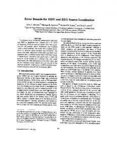
Our synthetic data consisted of corresponding pairs of dipole locations and sensor activations, as generated by our forward model. Given a dipole location and a set of sensor activations, the minimum error dipole moment can be calculated analytically. Therefore, we discarded the moment in all the experiments below. We made two datasets, one for training and the other for testing. Dipoles in the training and testing sets were drawn uniformly from truncated spherical regions, as shown in Figure 1. The dipole moments were drawn uniformly from vectors of strength ≤100 nAm. The corresponding sensor activations were the results of a forward model plus a noise model. To allow the network to interpolate rather than extrapolate, thus improving performance, the training set used dipoles from the larger region, while the test set contained only dipoles from the smaller inner region. We used a standard analytic forward model of quasistatic electromagnetic propagation in a spherical head [1, 6], with the sensor geometry of a 4D Neuroimaging Neuromag122 gradiometer. In order to properly compare the performance of localizers, we need a dataset for which we know the ground truth, but which contains the sorts of noise encountered in actual MEG recordings [5]. The real brain noise was taken from MEG recordings during periods in which the brain region of interest was quiescent. These signals were not averaged. The real brain noise has an RMS of roughly P n = 50–100 fT/cm. We measured the S/N ratio of a dataset using the ratios of the powers in the signal and
��������������� �� �� �� �� �� �� �� �� �� �� �� �� �� �� �� ��� ��������������� �� �� �� �� �� �� �� �� �� �� �� �� �� �� �� ��������������� �� � � � � � � � � � � � � � � � � � � � � � � � � � � � � ��������������� �� � � � � � � � � � � � � � � � � � � � � � � � � � � � � ��� ��������������� ��� �� �� �� �� �� �� �� �� �� �� �� �� �� �� ��������������� � �� �� �� �� �� �� �� �� �� �� �� �� �� �� ��������������� �� � � � � � � � � � � � � � � � � � � � � � � � � � � � � ��� Testing Region ��������������� �� � � � � � � � � � � � � � � � � � � � � � � � � � � � � ��������������� �� � � � � � � � � � � � � � � � � � � � � � � � � � � � � ��������������� �� � � � � � � � � � � � � � � � � � � � � � � � � � � � � ��� ��������������� �� �� �� �� �� �� �� �� �� �� �� �� �� �� �� ��������������� �� �� �� �� �� �� �� �� �� �� �� �� �� �� �� ��������������� �� � � � � � � � � � � � � � � � � � � � � � � � � � � � � ��� ��������������� �� � � � � � � � � � � � � � � � � � � � � � � � � � � � � ��������������� �� �� �� �� �� �� �� �� �� �� �� �� �� �� �� ��������������� �� � � � � � � � � � � � � � � � � � � � � � � � � � � � � � � � ��������������� �� � � � � � � � � � � � � � � � � � � � � � � � � � � � � ��������������� �� �� ��������������� �� ���� ���� ���� ���� ���� ���� ���� ���� ���� ���� ���� ���� ���� �����
the noise: S/N (in dB) = 10 log10 P s /P n where P s is the RMS (square root of mean square) of the sensor readings from the dipole and P n is the RMS of the sensor readings from the noise. The dataset was made by adding real brain noise (without scaling) to synthetic sensor activations generated by the forward model and exemplars whose resulting S/N ratio was under 0 dB were rejected.
9 cm 10 cm
2 cm 3 cm
Training Region
2.2
MLP structures
The Cartesian-MLP and the Soft-MLP charged with approximating the inverse mapping had an input layer of 122 units, one for each sensor. The Cartesian-MLP had two hidden layers with N1 and N2 units and an output layer of three units representing the dipole location (x, y, z). The Soft-MLP consists of one hidden layer with N units, and an output layer of 193 units representing the amplitudes of 193 uniformly distributed three-dimensional Gaussian functions in the training region of the head model [2]. These Gaussian functions are defined by � � |x − xi |2 for i = 1, . . . , 193 Gi (x) = exp − 2σ 2 where xi is a center of Gaussian function and σ is a fixed width parameter. These Gaussian functions are homogeneously distributed with adjacent centers at a distance 3 cm and a width parameter σ = 1.8 cm. The decoding strategy to convert the activations into a Cartesian coordinate representation was:
Spherical Head Model
Figure 1: Training and testing regions for a spherical head model. Bias Units 1
Output units had linear activation functions, while to accelerate training hidden units used the hyperbolic tangent activation function [7]. All units had bias inputs, adjacent layers were fully connected, and there were no cutthrough connections, which is shown in Figure 2. The 122 MEG sensor activations were scaled so that their RMS value was 0.5. The network weights were initialized with uniformly distributed random values in ±0.1. Backpropagation was used to calculate the gradient, and online stochastic gradient decent for the optimization. No momentum was used, and learning rate was chosen empirically. To empirically determine the number of hidden units, we trained two MLPs with various numbers of hidden units and we measured the tradeoff between approximation accuracy and computation time. Finally, we chose 122–60–30–3 and 122-80-193 as the Cartesian-MLP size and the Soft-MLP size, respectively.
Dipole Location x
1 −1
B1
1
y
1
z
−1
B2 −1
B3 Wij
B122
3 Units
122 Units
60 Units
30 Units
Cartesian−MLP structure Bias Units 1
1
MEG signals 1 0
B1
Dipole Location 1 0
B2
• For the 193 output values (ai ≈ Gi (x)), find the index i∗ of maximum amplitude i∗ = arg maxi ai . • For some neighborhood I of xi∗ , estimate the dipole location by linear interpolation, P a i xi ˆ = Pxi ∈I . x xi ∈I ai
1
1
MEG signals
Decoder 1
x y z
0
B3 Wij
1
B122
0
122 Units
80 Units
193 Units
Soft−MLP structure x1 x2 x3
Yj = tanh( Σ Wijxi)
x1 x2 x3 a
b
xn
xn
Activation Functions Model
b if s > b Σ Wijxi if a