Journal of the Korean Physical Society, Vol. 67, No. 12, December 2015, pp. 2026∼2032
Electromagnetic Metamaterial Simulations using a GPU-Accelerated FDTD Method Myung-Su Seok, Min-Gon Lee, SeokJae Yoo and Q-Han Park∗ Department of Physics, Korea University, Seoul 02841, Korea (Received 5 November 2015, in final form 25 November 2015) Metamaterials composed of artificial subwavelength structures exhibit extraordinary properties that cannot be found in nature. Designing artificial structures having exceptional properties plays a pivotal role in current metamaterial research. We present a new numerical simulation scheme for metamaterial research. The scheme is based on a graphic processing unit (GPU)-accelerated finitedifference time-domain (FDTD) method. The FDTD computation can be significantly accelerated when GPUs are used instead of only central processing units (CPUs). We explain how the fast FDTD simulation of large-scale metamaterials can be achieved through communication optimization in a heterogeneous CPU/GPU-based computer cluster. Our method also includes various advanced FDTD techniques: the non-uniform grid technique, the total-field/scattered-field (TFSF) technique, the auxiliary field technique for dispersive materials, the running discrete Fourier transform, and the complex structure setting. We demonstrate the power of our new FDTD simulation scheme by simulating the negative refraction of light in a coaxial waveguide metamaterial. PACS numbers: 02.70.Bf, 78.20.Bh Keywords: FDTD, GPU, Electromagnetic simulations, Metamaterials DOI: 10.3938/jkps.67.2026
I. INTRODUCTION The finite-difference time-domain (FDTD) method is a numerical technique to solve Maxwell’s equations discretized in the space- and the time-domain [1, 2]. The FDTD method directly solves Maxwell’s equations in the time domain. This allows a spectral analysis of the electromagnetic system over a wide spectral range in a single run by employing a short-time pulse as the source. The spectral advantage and the simplicity of the method makes the FDTD method a primary tool for designing metamaterials and plasmonic devices [3–9]. However, the FDTD method is computationally expensive as it requires electric and magnetic vector field components at each grid points in the computational domain whereas a quite large number of grid points is needed for the stability of the numerical calculation. Recent advances in metamaterial research demand ever increasing computational power in terms of memory and speed for a largescale simulation of subwavelength structures. Therefore, a fast and efficient computational scheme for large-scale FDTD simulations is highly desired for metamaterial research. In this paper, we introduce a GPU-accelerated FDTD method for metamaterial simulations. The main features of our method include an acceleration of the computa∗ E-mail:
[email protected]; Fax: +82-2-3290-3969
tion by using a GPU and an optimization of the communication between nodes in a CPU/GPU-heterogeneous computer cluster. GPUs are highly efficient for scientific computations because they are specialized for parallel computations [10]. By adopting our GPU-accelerated FDTD computational scheme, we obtain a 10-fold increase in computational speed compared to the conventional FDTD computation using a CPU. By optimizing the communication between nodes in a computer cluster, we reach the theoretical upper limit of performance of the FDTD computation. Open-source software for our method, named as the Korea University’s Electromagnetic wave Propagator (KEMP), is presented in this paper; it is also available online [11,12]. KEMP possesses various advanced FDTD functionalities, with which we demonstrate the negative refraction of light inside a coaxial waveguide metamaterial by using the FDTD simulations in KEMP.
II. OPTIMAZATION OF GPU-ACCELERATED FDTD COMPUTATION Large-scale simulations of metamaterials require a significant increase in computational speed for the FDTD method. Such a speed-improvement can be achieved by using GPU acceleration and computer clusters. Origi-
-2026-
Electromagnetic Metamaterial Simulations using a GPU-Accelerated FDTD Method – Myung-Su Seok et al.
-2027-
Table 1. Experimental performances of the FDTD computations using KEMP on various devices. For the FDTD computation on GPUs, experimental performances are compared to the theoretical upper limit of the FDTD computation performances. Device Intel Core i7-6700 (CPU) Intel Core i7-3930K (CPU) NVIDIA Tesla C2075 (GPU)
KEMP performance (GFLOPS) 7.42 9.12 27.53
Theoretical upper limits (GFLOPS) 9.60 12.57 29.02
Achievement (%) 78.2 77.5 94.9
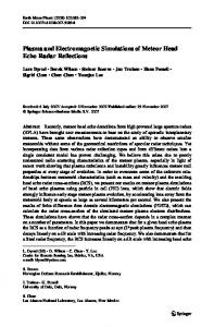
Fig. 1. (Color online) (a) Conventional non-optimized communications and corresponding timeline for the computation of the divided domains (green) and boundary surfaces (yellow), and communications between computers (black) in a CPU cluster and a GPU cluster. (b) Communications optimized by using the host-buffer method, and corresponding timeline in a CPU/GPU heterogeneous cluster. Scale bars for the timelines are 5 ms.
nally, GPUs have been developed for image processing using computers, but they are also highly efficient for parallel computations. In the FDTD method, most computations are elementary arithmetic, and a GPU with many cores is better suited for this purpose and for increasing the computational speed [10]. Using both of the GPU acceleration and computer clusters, we can significantly accelerate the computational speed of the FDTD method. Recently, we created an open-source software realizing our GPU-accelerated FDTD method, named as the Korea University’s Electromagnetic wave Propagator (KEMP), and posted it online. KEMP supports both the CPU and the GPU computations of the FDTD method with various functionalities. Table 1 shows performance tests of the FDTD computation using KEMP operating on Intel CPUs and NVIDIA GPUs. The performance of the FDTD computation is measured by using GFLOPS, the number of giga floating-point operations per second. We can achieve a performance enhancement of 301 ∼ 669% when we operate KEMP using GPUs in comparison to using CPUs. In
Table 1, the theoretical upper limit for the FDTD computation is determined by using the memory bandwidth of each device because the amount of memory access is much higher than the number of floating point operations for the FDTD method [13]. We find that experimental performances of the FDTD computation using KEMP nearly reach the theoretical upper limit of each device in Table 1. KEMP also includes the FDTD computation on a CPU/GPU-heterogeneous computer cluster, which is composed of multiple nodes equipped with CPUs and GPUs. Using the host-buffer method [14] to shorten the total execution time of the FDTD method, we optimize the communication between nodes in the cluster. Figure 1(a) shows the schematic of the conventional nonoptimized communications. In the conventional communication, the total computation domain is divided by the number of nodes in a cluster. At the boundary surface (yellow region in Fig. 1) of each divided domains (green region in Fig. 1), nodes communicate with each other and exchange calculated data. For a CPU cluster (two nodes
-2028-
Journal of the Korean Physical Society, Vol. 67, No. 12, December 2015
Fig. 2. (Color online) Throughput of the FDTD computation corresponding to the number of nodes. Black, red, and blue lines are the ideal zero-time communications (black), the non-optimized communications (red), and the communications optimized by using the host-buffer method (blue).
with Intel i7-4770 CPUs), the computation time of the each divided domain (green and yellow bars) is a dominant contribution to the total execution time rather than the communication time (black bar). For a GPU cluster, the computation time and the communication time are comparable because the GPU acceleration significantly shortens the computation time. Note that the communication time is invariant to CPUs and GPUs. Figure 1(b) shows the optimization of communications by using the host-buffer method. When the host-buffer method is used, communications and computations are simultaneously done by both of the CPUs and the GPUs, as shown in the timeline in Fig. 1(b). As a result, most of the communication time is effectively hidden behind the computation time. In Fig. 1(b), we find that the FDTD computation in a CPU/GPU heterogeneous cluster (two nodes with Intel i7-4770 CPUs and NVIDIA GTX Titan Black GPUs) can shorten the total computation time rather than the conventional communications in a GPU cluster (Fig. 1(a)). Figure 2 shows the throughput of the FDTD computation in terms of number of nodes. The throughput of the FDTD computations on computer clusters is measured by using the GFLOPS in Fig. 2. Each node in the cluster uses an Intel i7-4770 CPU and a NVIDIA GTX Titan Black GPU. In the ideal case of zero-time communications, the total throughput increases linearly with the number of nodes. We find marked declines of the throughput for non-optimized communications due to a bottleneck of the communication time in the cluster. When the host-buffer method is used, the throughput of the FDTD computation on the CPU/GPU heterogeneous cluster approaches the upper limit of the ideal case. This makes possible to fast simulations of largescale electromagnetic problems.
Figure 3 shows a diagram of the file structure in the KEMP. In Fig. 3, we group the files of the KEMP according to their functionalities. By the order of the user interface file (“kemp test.py” in Fig. 3), the file group “Main” executes the actual FDTD computations by using the group “Engine”, which includes the GPU acceleration of the FDTD computations. During the FDTD computations, the “Main” group calls various advanced techniques of the FDTD method from other groups. The “Materials” group assigns material information for arbitrary structures in the computation domain. Using “dipersive.py” in the “Materials” group, the KEMP supports the dispersion of materials by using the Drude critical point (Drude-CP) model [15], and prepared datasets of material dispersion for the Drude-CP model can be found in the folder “material data/”. The “Utility” group includes the excitation of the source (“incident.py”) and the running Fourier transform (“rft.py”). The “Domain” group controls the computation domain in the FDTD method, and it provides the perfectly matched layer (PML) and the periodic boundary condition (PBC) on the boundary of the computation domain. The PML corresponds to the Sommerfeld radiation boundary condition as |r| → ∞ by absorbing all electromagnetic waves at the PML boundaries [16, 17]. The PBC realizes the infinitely-repeated computation domain [2]. The “User interface” group presents the functionalities of the unit conversion (“units.py”) and displays error massages (“exception.py”) and data input/output (“managedata.py”). The user interface of the KEMP is based on the python programming language. It should be noted that the user interface script file corresponds to “kemp test.py” in Fig. 4. Figures 4 and 5 show the user interface that measures the transmission and the reflection of a thin gold slab with a 5-nm thickness. The first block of the user interface in Fig. 4 imports KEMP modules and required python modules from the library. Required python modules for the user interface, numpy, scipy, matplotlib, and h5py, respectively, provide the base N-dimensional array package, the scientific computing package, the plotting library, and the HDF5 binary data format package. The second block in Fig. 4 shows settings of the computation domain. The size of each grid is defined by the declaration “dx, dy, dz = [.1*nm, .1*nm, .1*nm]” while numbers of grids along x-, y-, and z-axis are defined by the declaration “nx, ny, nz = [5, 5, 20000]”. KEMP supports both 2-dimensional (2D) and 3-dimensional FDTD (3D) computations. For the 2D computation, we can use the transverse electric (TE) and transverse magnetic (TM) modes. The KEMP uses Cartesian coordinates for the discretized grids, and three 1-dimensional arrays define sizes of the grids. The function ”KEMP. FDTDspace(mode, space grid, data type, engine name, device ids, MPI extension)” controls these options regarding the computation domain. The third block defines the boundary condition of the computation domain. We can use PML or PBC
Electromagnetic Metamaterial Simulations using a GPU-Accelerated FDTD Method – Myung-Su Seok et al.
-2029-
Fig. 3. File structure diagram of KEMP.
Fig. 4. (Color online) The first half of the user interface in KEMP.
on the outermost boundary of the computation domain. In Fig. 4, only surfaces normal to the zaxis are declared as PMLs due to the declaration “pml apply(applied boundary planes)”. In the declaration “pbc apply(applied axes)”, the option of the axis “True” activates the PBC along surfaces to the axis, while the option “False” deactivates the PBC. Structures and objects for the FDTD simulation are designated in the fourth block in Fig. 5. Function “stc.Box(material, coordinate)” creates the geometry of the box of the designated material at the designated position. In the KEMP, other functions creating complex
geometries are supported: ellipsoids, spheres, cylinders, cones, polyprisms, polypyramids, and their arbitrary rotations. Function “fdtd.apply direct source(field name, apply region)” in the sixth block designates the polarization, position, and type of an electromagnetic source. In Fig. 5, the launching position of the plane wave is located at the surface of z = +5000. The last block in Fig. 5 illustrates the execution of the FDTD computation. In the for-statement, we execute the FDTD computation until “tstep” reaches “tmax”. We set “tmax” as 80000 to compute the FDTDs for five periods of 800-nm
-2030-
Journal of the Korean Physical Society, Vol. 67, No. 12, December 2015
Fig. 5. (Color online) The second half of the user interface in KEMP.
wavelength.
III. METAMATERIAL SIMULATIONS We demonstrate the large-scale FDTD simulation of the negative refraction of light in a metamaterial by using KEMP. For testing the FDTD simulation of the negative refraction, we use a hexagonal array of subwavelength coaxial waveguides in a silver film [18]. Figure 6(a) shows a schematic drawing of the negative-index coaxial waveguide metamaterial. The annular channels of the coaxial waveguides are filled with GaP. The inner radius r1 and the outer radius r2 of the silver cores are 37.5 nm and 62.5 nm, respectively. The periods of the hexagonal array are, respectively, px = 165 nm and py = 286 nm along the x- and the y-axis. The permittivity values of silver and GaP are taken from tabulated data [19,20]. Figure 6(b) illustrates the negative refraction of light at a wavelength of λ = 480 nm inside the coaxial waveguide metamaterial whose thickness is 1000 nm. Light with the angle of incidence of θi = 30◦ impinges on the metamaterial, and we find the angle of refraction to be θr = −36.9◦ . By Snell’s law, we find that the effective refractive index of the metamaterial in Fig. 6(b) is −0.83. For the FDTD simulation in Fig. 6(b), we use a total of 1.28 × 10⁹ grids because the thickness of the coaxial
waveguide metamaterial in the computation domain in Fig. 6(b) is much larger than the wavelength of light. We use a heterogeneous CPU/GPU-based computer cluster composed of 11 nodes with 1 CPU (Intel i7-4770) and 2 GPUs (NVIDIA Tesla C2075) for the FDTD simulation in Fig. 6(b). When we use both CPUs and GPUs operated by using the KEMP, we find a 480% enhancement in the computation speed in comparison with using only CPUs. In Fig. 6(c) and (d), we also extract the effective refractive index of the coaxial waveguide metamaterial with a thickness of 100 nm by using the parameter retrieval method [21]. Figure 6(c) shows the reflectance and the transmittance spectra of the coaxial waveguide metamaterial, and the transmission mode is found in the spectral range near 470 nm. In Fig. 6(d), we achieve a negative effective index of nef f = −1.45 at a wavelength of 489 nm by using the coaxial waveguide metamaterial.
IV. CONCLUSION In conclusion, we presented KEMP, the GPUaccelerated open-source software for the FDTD method. KEMP is distributed at our group website [11] and sourceforge [12], which is a web-based repository of open-source software. KEMP supports not only the GPU acceleration of the FDTD computation but also
Electromagnetic Metamaterial Simulations using a GPU-Accelerated FDTD Method – Myung-Su Seok et al.
-2031-
Fig. 6. (Color online) (a) Negative-index coaxial waveguide metamaterial. (b) Negative refraction of light at a wavelength of λ = 480 nm inside a coaxial waveguide metamaterial with a thickness of 1000 nm. (c) Spectra for the reflectance (black) and the transmittance (red), and (d) corresponding spectra for the real (black) and the imaginary parts (red) of the effective refractive index of a coaxial waveguide metamaterial with a thickness of 100 nm.
the FDTD computation using a CPU/GPU heterogeneous computer cluster system. KEMP also includes the non-uniform grid technique, the total-field/scatteredfield (TFSF) technique, the auxiliary field technique for dispersive materials, the running discrete Fourier transform, and the complex structure setting, and we expect KEMP to become a powerful tool for designing and studying metamaterials and plasmonic devices.
ACKNOWLEDGMENTS This research was supported by the NanoMaterial Technology Development Program through the National Research Foundation of Korea (NRF) funded by The Ministry of Science, ICT & Future Planning (MSIP) (No. 2011-0020205) and by the Center for Advanced Meta-Materials (CAMM) funded by the Ministry of Science, ICT and Future Planning as a Global Frontier Project (CAMM-2014M3A6B3063710).
REFERENCES [1] K. Yee, IEEE Trans. 14, 302 (1966).
[2] Taflove and S. Hagness, The Finite-Difference TimeDomain Method, 3rd ed. (Artech House, Boston and London, 2005). [3] J. Choe, J. Kang, D. Kim and Q. Park, Opt. Express 20, 6521 (2012). [4] S. Yoo and Q.-H. Park, Opt. Express 20, 16480 (2012). [5] W. Choi, Q.-H. Park and W. Choi, Opt. Express 20, 20721 (2012). [6] K.-H. Kim and Q.-H. Park, Sci. Rep. 3, 1062 (2013). [7] J.-H. Kang and Q.-H. Park, Sci. Rep. 3, 1 (2013). [8] S. Yoo, M. Cho and Q.-H. Park, Phys. Rev. B 89, 161405 (2014). [9] S. Yoo and Q.-H. Park, Phys. Rev. Lett. 114, 203003 (2015). [10] S. E. Krakiwsky, L. E. Turner and M. M. Okoniewski, Proc. IEEE MTT-S Int. Microw. Symp. Dig. 2, 1033 (2004). [11] Nano Optics Lab. http://nol.korea.ac.kr/. [12] KEMP project page in Sourceforge. http://kemp.sourceforge.net/. [13] K.-H. Kim, K. Kim and Q.-H. Park, Comput. Phys. Commun. 182, 1201 (2011). [14] K.-H. Kim and Q.-H. Park, Comput. Phys. Commun. 183, 2364 (2012). [15] A. Vial and T. Laroche, J. Phys. D, Appl. Phys. 40, 7152 (2007). [16] J. P. Berenger, J. Comput. Phys. 114, 185 (1994). [17] J. A. Roden and S. D. Gedney, Microw. Opt. Technol. Lett. 27, 334 (2000). [18] S. P. Burgos, R. de Waele, A. Polman and H. A. Atwater,
-2032-
Journal of the Korean Physical Society, Vol. 67, No. 12, December 2015
Nat. Mater. 9, 407 (2010). [19] P. B. Johnson and R. W. Christry, Phys. Rev. B 6, 4370 (1972). [20] E. D. Palik and G. Ghosh, Handbook of Optical Con-
stants of Solids (Academic Press, San Diego, 1985). [21] D. R. Smith, D. C. Vier, T. Koschny and C. M. Soukoulis, Phys. Rev. E 71, 036617 (2005).