Electromagnetically induced transparency and dynamic Stark effect in

Electromagnetically induced transparency and dynamic Stark effect in coupled quantum resonators M. A. de Ponte, C. J. Villas-Bˆoas, R. M. Serra, and M. H. Y. Moussa Departamento de F´ısica, Universidade Federal de S˜ ao Carlos, P.O. Box 676, S˜ ao Carlos, 13565-905, S˜ ao Paulo, Brazil

arXiv:quant-ph/0411087v2 13 Dec 2004

In this work we reproduce the phenomenology of the electromagnetically induced transparency and dynamic Stark effect in a dissipative system composed by two coupled bosonic fields under linear and nonlinear amplification process. Such a system can be used as a quantum switch in networks of oscillators. PACS number: 32.80.-t, 42.50.Ct, 42.50.Dv

Much of the recent work in quantum optics has been devoted to quantum coherence and interference as a result of the mastery gained in manipulating atom-field interaction, which allows us to probe fundamental quantum effects. Within this scenario, electromagneticallyinduced transparency (EIT) [1] plays an essential role in a variety of processes, ranging from lasing without inversion [2] and enhanced nonlinear optics [3] to quantum computation and communication [4]. Relying on destructive quantum interference, EIT is a phenomenon in which the absorption of a probe-laser field resonant with an atomic transition is reduced or even eliminated by the application of a strong driving laser to an adjacent transition. This effect can be understood as arising from the ac-Stark splitting of an excited atomic state linking the two adjacent transitions. When the splitting is smaller than the excited state width, the two resulting levels are indistinguishable, leading to a destructive interference in the probe absorption spectrum [1]. As the intensity of the driving field increases, the splitting is enlarged, eliminating the indistinguishability and, consequently, the absorption spectrum evolves to the AutlerTownes (AT) doublet. By a similar mechanism, although relying on nonlinear interactions, the strong excitation of a two-level atom induces a dynamic Stark effect (DSE) leading to the appearance of sidebands in the resonance fluorescence spectrum [5]. Recently, some effects of three-level atom optics, including EIT, were simulated [6] via the tunneling interaction in the context of trapped atoms. In this connection, the phenomenology observed in EIT was reproduced in a system of two coupled dissipative classical oscillators in Ref. [7]. One of these oscillators, modeling the threelevel atom, is subject to a linear driving force [7] playing the role of the probe field. The pump field is simulated by the coupling between the oscillators. The quantum version of this classical analog of EIT, which helps to deepen our understanding of this phenomenon and its properties, will be analyzed in the present work. Here, the classical oscillators are replaced by two quantum resonators interacting through a Josephson-type coupling. Linear and nonlinear amplifications are employed as the probe fields, the former is used to emulated the EIT phe-

nomenon, and the latter is applied to obtain the DSE — reproducing the phenomenology of the nonlinear mechanism related to resonance fluorescence from a stronglydriven two-level transition. The coupling parameter between the resonators plays the role of the driving field, by analogy with the standard EIT and DSE. We show that the signatures of these processes can be obtained by measuring the field quadratures. The Hamiltonian of the coupled dissipative resonators, labeled by ℓ = 1, 2, is given by (~ = 1) H=

X

ωℓ a†ℓ aℓ +

ℓ

X

ωℓk b†ℓk bℓk

ℓ,k

   X Vℓk aℓ b†ℓk + a†ℓ bℓk + λ a1 a†2 + a†1 a2 + 

+̥



ℓ,k

e−iνt a†1

p

+ e iνt a1


p



,

(1)

where a†ℓ (aℓ ) is the creation (annihilation) operator for the oscillator mode ℓ of frequency ωℓ , whereas b†ℓk (bℓk ) is the analogous operator for the kth bath mode of oscillator ℓ, whose corresponding frequency and coupling strength are ωℓk and Vℓk , respectively. The coupling strength between the oscillators is λ and the classical driving field applied to oscillator 1 has intensity ̥ and frequency pν, with the parameter p = 1 or 2 for the linear or nonlinear amplification process. Following the reasoning in Ref. [8], we obtain (in a rotating frame with frequency ν and assuming the reservoir at zero temperature) the master equation for the system dynamics, given by dρ12 (t) = i [ρ12 (t) , H0 ] dt i h i X Γℓ h + aℓ ρ12 (t) , a†ℓ + aℓ , ρ12 (t) a†ℓ , 2 ℓ

(2)

where Γℓ is the damping rate of resonator ℓ and we have

2 defined H0 ≡

X ℓ

+̥

  Ωℓ a†ℓ aℓ + λ a1 a†2 + a†1 a2

   p p a†1 + (a1 ) ,

(3)

with Ωℓ ≡ ωℓ − ν being the effective frequency of the oscillator ℓ shifted by the amplification process. Using the standard procedures and assuming Markovian white noise, we derive a c-number version of the master equation (2) for the symmetric ordered characteristic function χ({ηℓ } , t), given by   ∂ dχ({ηℓ } , t) X + c.c. = Cℓ ({ηℓ }) dt ∂ηℓ ℓ i (p−1) +i̥ (η1 + η1∗ ) (η1 − η1∗ ) δℓ,1 × χ({ηℓ } , t),

(4)

where Cℓ ({ηℓ }) = ηℓ Λℓ + iληℓ−(−1)ℓ + 2i (p − 1) ̥η1∗ , Λℓ = Γℓ /2 + iΩℓ , and ηℓ is the complex parameter of the characteristic function. From the analytical solution of Eq. (4), obtained by standard techniques [8], we observe for the linear amplification (p = 1), that the modes in both resonators always evolve to stationary coherent states, characterized by the equilibrium between the amplification process and the dissipative mechanisms, mediated by the coupling strength λ. These stationary coherent states, |αi1 and |βi2
, have the complex amplitudes
α = −i̥Λ2 / λ2 + Λ1 Λ2 and β = −λ̥/ λ2 + Λ1 Λ2 . The EIT-like phenomenon, which occurs in the region where Γ1 ≫ λ ≫ Γ2 , is characterized by the state of the field in resonator 1 around the relaxation time τR of the joint system. For the linear amplification case, the relaxation time, derived from the condition ∂χ({ηℓ } , t)/∂t → 0 [8], is given by the simple expression τR = 2λ2 /Γ1 + Γ2 /2. In Ref. [8], it is noted that the cavity-field states are interchanged between the resonators through state-swap and the state-recurrence dynamics. Before the relaxation time, the coherence dynamics of quantum states between the two resonators prevents the EIT from occurring. Therefore, the system must achieve a stationary state to enable the appearance of the destructive interference, which promotes the EIT. For this reason, from here on we will be interested in the states of resonator 1 around the relaxation time. In atomic samples the EIT phenomenon is characterized by the permittivity of the medium, associated with the complex quantity n + ik, where the dispersive and the absorptive responses follow, respectively, from the real part of the refractive index n and the absorption coefficient k [9]. Here, the role of the permittivity is 1/2 played by the quantity Eℓ eiΘℓ representing the center of the quasi-probability distribution of the cavity-field state in the phase space defined by its quadratures Xℓ =

    aℓ + a†ℓ /2 and Yℓ = aℓ − a†ℓ /2i. The absorption coefficient is directly associated with the mean energy of the cavity field  ℓ, given by the correlation function Eℓ = Xℓ2 + Yℓ2 (in units of ~ωℓ ). The dispersive response is associated with the angle Θ through the correlation function hXℓ Yℓ + Yℓ Xℓ i /Eℓ = sin (2Θℓ ). In Ref. [7] the dispersive response Re [x1 (e ω−ω e1 )] is derived from the real part of the frequency dependence of the amplitude x1 (e ω −ω e1 ) of one oscillator (frequency ω e1 ), submitted to a linear driving force (frequency ω e ), and coupled to another oscillator (frequency ω e2 and amplitude x2 ). In the present model, the equivalent mean value hYℓ i also leads to the required dispersive response, as in [7], for the linear amplification process (p = 1). However, in the case of nonlinear amplification (p = 2), the mean value hYℓ i is not a convenient quantity to measure the dispersive response since it is null when the initial excitation of the cavity field ℓ is also null (vacuum state). To circumvent this problem, we have considered the correlation function hXℓ Yℓ + Yℓ Xℓ i /Eℓ to describe the dispersive response in a quite general way. In fact, its classical analog, proportional to Re [xℓ pℓ ] (where pℓ is the momentum of the classical oscillator ℓ), also leads to the usual dispersion exhibiting a very steep slope in the EIT regime. The absorptive and dispersive responses given by the corre

 lation functions Xℓ2 + Yℓ2 and hXℓ Yℓ + Yℓ Xℓ i /Eℓ , respectively, are computed from the characteristic function χ({ηm } , t) (m = 1, 2) as ∂2 χ({η } , t) , (5a) Eℓ = − m ∗ ∂ηℓ ∂ηℓ ηm →0 ! ∂2 1 ∂2 sin (2Θℓ ) = χ({η } , t) − . m 2 ∗ Eℓ ∂ (ηℓ )2 ∂ (ηℓ ) η →0 m

(5b)

Linear amplification. To characterize the EIT, we plot the mean values E1 and sin (2Θ1 ), for resonator 1, against the detuning ∆ = (ν − ω1 ) /Γ1 . Before the relaxation time (τR ), i.e., t ≪ τR , the EIT is inhibited by the coherence dynamics between the cavity-field states. Near the relaxation time, the EIT starts appearing, evolving to its standard shape at the relaxation time, as displayed in Fig. 1(a). In Fig. 1(b) we assume the non-degenerate case ω1 = ω2 − ǫ at the relaxation time, where the hole burned when ν = ω1 in the degenerate case [Fig. 1(a)], shifts to ν = ω1 + ǫ (where ǫ/Γ1 = 3). It is interesting to note, that in the non-degenerate case [Fig. 1(b)], the EIT happens when the linear amplification (ν) is in resonance with resonator 2 (ω2 ). A complete transparency occurs only when Γ2 = 0, since the minimum of the hole burned in the peak of the absorptive response is given
2  by E1min = 2̥Γ2 / 4λ2 + Γ1 Γ2 . Assuming the same parameters as those in Fig. 1(a) but a stronger coupling strength (λ/Γ1 = 1), the EIT evolves to the AT regime as shown in Fig. 1(c). Finally, the dispersion curves, in

3 0.25

0.15

0.00 -2

0

( ν - ω1 ) / Γ1

2

0.15

0

( ν - ω1 ) / Γ1

ν = ω2

2

-0.25 -2

0

( ν - ω1 ) / Γ1

0.30

ν = ω2

2

ε1 / ε0 0.03

8

0 -3 -6x10

0 -3 -6x10

-3

0 ( ν - ω1 ) / Γ1

6x10

0.00

0.07

1.0 c)

0 ( ν - ω1 ) / Γ1

-3

6x10

d) 0.5

0.0 -0.07

( ν - ω1 ) / Γ1

ε1

0.25 c)

0.15

0.00 -4

0.00 ( ν - ω1 ) / Γ1

16

0.00

b)

100

0.0 -0.03

ε1 / ε0

sin (2 Θ1)

b)

0.00 -2

0 ( ν - ω1 ) / Γ1

0.25

ε1

0.30

200 a)

0.9

0.00

-0.25 -2

2

1.8

ε1 / ε0

sin (2 Θ1)

ε1

a)

ε1 / ε0

0.30

0.00

0

( ν - ω1 ) / Γ1

4

-0.25 -4

0

( ν - ω1 ) / Γ1

FIG. 1: Absorptive-like (left side) and dispersive-like (right side) curves for the linear amplification process (at t = τR ) assuming: (a) the degenerate case (ω1 = ω2 ) and Γ2 ≪ λ ≪ Γ1 , (b) the non-degenerate case (ω1 = ω2 − ǫ),. (c) the degenerate case and Γ2 ≪ λ ≈ Γ1 . To plot these figures we have assumed the following parameters: Γ2 /Γ1 = 10−4 and ̥/Γ1 = 1/4. For (a) and (b) we have used λ/Γ1 = 2 × 10−2 and for (c) λ/Γ1 = 1.

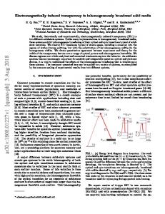
the right side of Fig. 1(a,b,c), display the well-known signature of the EIT effect. Nonlinear amplification. In the nonlinear or parametric amplification case (p = 2), there is a well-known threshold in the dynamics of the system [10, 11] which is reached when the rescaled amplification parameter, ξ = 4̥/Γ1 , equals the critical value ξc (which depends on the critical amplification amplitude ̥c ). We obtain three different dynamics for the solutions of Eq. (4), which depend on whether the rescaled amplification is strong (ξ > ξc ), critical (ξ = ξc ), or weak (ξ < ξc ). When ξ ≥ ξc the asymptotic solution diverges for any physical quantity whereas we obtain stationary solutions when ξ < ξc . In the degenerate resonance case, ω1 = ω2 = ω, the critical amplification parameter is given either by ξc = 1 + 4λ2 / (Γ1 Γ2 ) (if λ < Γ2 /2) or ξc = 1 + Γ2 /Γ1 (if λ ≥ Γ2 /2). Evidently, when λ = 0 we recover the usual result ξc = 1 for an uncoupled system under nonlinear amplification. In these three regimes the state of oscillator 1 evolves to a squeezed coherent state (SCS) which is stationary for ξ < ξc and whose energies increase monotonically for ξ ≥ ξc . Now, in order to analyze the behavior of the absorp-

4

FIG. 2: Absorptive-like curves for the nonlinear amplification process (ω1 = ω2 ): in (a) the weak regime (ξ = ξc −1.5×10−4 , ξc = 1 + 10−4 ), (b) critical regime (ξ = ξc ), (c) strong regime (ξ = ξc + 1, 5 × 10−4 ), and (d) in the weak amplification regime at the relaxation time τeR , but increasing the coupling strength. To plot these figures we have assumed the following parameter: Γ2 /Γ1 = 10−4 . For (a-c) we have used λ/Γ1 = 5 × 10−5 and for (d) we have used λ/Γ1 = 10−2 . Where the dotted line is for t = 0.8 × τeR , the solid line is for t = τeR , the dashed line is for t = 1.1 × τeR , and we have assumed the vacuum states as initial states for the resonators 1 and 2.

tive and dispersive curves of resonator 1, in the three regimes exposed above, we plot the rate E1 /E, instead of E1 , where E stands for the value of E1 when the detuning ∆ = 0. In this case, the EIT occurs only in a narrow interval |ξ| . ξc + 10−4 around the threshold given by the critical parameter ξc , i.e., around ̥c = (Γ1 + 4λ2 /Γ2 )/4 for λ < Γ2 /2, or ̥c = (Γ1 + Γ2 )/4 for λ ≥ Γ2 /2. Differently from the linear amplification process, where the EIT can be achieved independently of the ratio ̥/Γ1 , the strong dependence of this effect upon the amplitude of the nonlinear driving field follows from the two-photon nature of this amplification process. As far as the coupling strength is concerned, although it must be much smaller than Γ1 as in the linear amplification case, here it can be around Γ2 , obeying the relation Γ2 . λ ≪ Γ1 . In the nonlinear case the relaxation time τeR can only be obtained from the condition ∂χ({ηℓ } , t)/∂t → 0 in the weak amplification regime. This time will be used as a reference to compare the three different amplification regimes, since there is no stationary dynamics when ξ ≥ ξc . We can see in Fig. 2(a), the absorptive curve for the weak amplification regime, that the EIT is not so pronounced as in the linear amplification case. In fact, it can barely be characterized as an EIT, since the maximum of the ratio E1 /E0 is close to unity (i.e., the minimum of the hole burned in the peak of the absorptive curve, when ∆ = 0). The absorptive curve remains immovable for t > τeR due to the stationary solution achieved in the

4 weak amplification regime. Differently from Fig. 2(a), we observe that in the critical regime, Fig. 2(b), the maximum of the ratio E1 /E is about two orders of magnitude larger than unity (E1 = E) for t = τeR (solid line), increasing as time goes on. However, as in the weak amplification regime, the behavior observed here can hardly be characterized as an EIT, but rather a mixing of EIT and AT effects, since the hole burned in the peak of the absorptive response presents a significant width compared to the usual EIT. In Fig. 2(c), for the strong amplification regime, a mixing of the EIT and the AT effects is observed again, but the ratio E1 /E does not increase as quickly as in the critical regime — even so, E1 and E increase, independently, as faster as they do in the critical regime. The maximum of the rate E1 /E is (only) about one order of magnitude larger than unity (E1 = E) for t = τeR and increases as the time goes on. We note that the range of the detuning ∆, in Figs. 2(b) and (c) — where the absorptive curves assume significant values— is considerably smaller than that in Fig. 2(a) for the weak regime. Therefore, as the rescaled amplification parameter ξ increases, the range ∆ of the absorptive curve decreases. From this perspective, it is not difficult to understand why the range ∆ of the absorptive curve in the linear amplification regime (Fig. 1) is larger than those in the nonlinear one. Regarding the dispersive curve, it happens to be practically the same for the three parametric amplification regimes and the steep slope characteristic of the EIT effect is lost. Finally, in Fig. 2(d) we display the absorptive curve in the weak amplification regime at the relaxation time τeR , but increasing the coupling strength such that λ/Γ1 = 10−2 (instead of 5 × 10−5 ). We thus observe the wellknown pattern exhibited by the resonance fluorescence spectrum of a two-level atom driven by an incident field whose Rabi frequency is comparable to, or larger than, the atomic linewidth. After all, as the phenomenology of the EIT can be reproduced in a system of two coupled dissipative oscillators, the same occurs with the phenomenology of resonance fluorescence. Resonator 1 again plays the role of the two-level atom, while the strong driving field (whose intensity leads to a modulation of the quantum dipole moment inducing sidebands in the spectrum [12]) is simulated by the nonlinear amplification together with resonator 2. In fact, high-intensity driving fields give rise to nonlinear interactions which may be attributed to two laser fields [13], modeled by the actual parametric field plus resonator 2. The pattern displayed in Fig. 2(d) can also be obtained in the critical and strong amplification regimes but, of course, it does not occur with linear amplification, whatever its intensity. The parametric amplification field is the only nonlinear ingredient in our system of two coupled dissipative oscillators. We have shown that a system of two coupled dissipative oscillators, under linear and parametric amplifi-

cation, can reproduce the phenomenology of EIT and DSE, respectively. Such phenomena can be, at principle, implemented in several physical contexts, such as: cavity quantum electrodynamics [14], trapped ions [15], and nanomechanical oscillators [16]. The system presented here can be used for quantum switching purposes, since the hole burned in the EIT regime can be shifted by external means, feeding or draining the field in resonator 1. For example, the dispersive interaction of a fermionic particle with the field in oscillator 2 can pull both oscillators out of resonance, changing the profile of the absorption curve of oscillator 1 from Fig. 1(a) to 1(b). Therefore, these effects have the potential to be used as a control mechanism in networks of quantum oscillators, a subject which attracts great attention nowadays [17]. This work was supported by FAPESP and CNPq, Brazilian agencies. We also thank Profs. P. Nussenzveig and B. Baseia for helpful discussions.

[1] S. E. Harris, Phys. Today 50(7), 37 (1997); J. P. Marangos, J. Mod. Opt. 45, 471 (1998). [2] A. S. Zibrov et al., Phys. Rev. Lett. 75, 1499 (1995). [3] S. E. Harris, J. E. Field, and A. Imamoglu, Phys. Rev. Lett. 64, 1107 (1990); H. Schmidt and A. Imamoglu, Opt. Lett., 21 1936 (1996); S. E. Harris and L. V. Hau, Phys. Rev. Lett. 82, 4611 (1999); M. D. Lukin and A. Imamoglu, Phys. Rev. Lett. 84, 1419 (2000). [4] M. D. Lukin, S. F. Yelin, and M. Fleischhauer, Phys. Rev. Lett. 84, 4232 (2000); M. D. Lukin and A. Imamoglu, Nature (London) 413, 273 (2001); Z. Ficek and S. Swain, J. Mod. Opt. 49, 3 (2002). [5] B. R. Mollow, Phys. Rev. 188, 1969 (1969); R. E. Grove, F. Y. Wu, and S. Ezekiel, Phys. Rev. Lett. 35, 1426 (1975); W. Hartig et al., Z. Physik A 278, 205 (1976). [6] K. Eckert et al., Phy. Rev. A 70, 023606 (2004). [7] C. L. Garrido Alzar, M. A. G. Martinez, and P. Nussenzveig, Am. J. Phys. 70, 37 (2002). [8] M. A. de Ponte, M. C. de Oliveira, and M. H. Y. Moussa, e-print quant-ph/0309082. [9] L.-M. Duan et al., Nature 414, 413 (2001); A. Kuzmich et al., Nature 423, 731 (2003). [10] H. J. Carmichael, G. J. Milburn, and D. F. Walls, J. Phys. A: Math Gen. 17, 469 (1984). [11] S. S. Mizrahi, M. H. Y. Moussa, and B. Baseia, Int. J. Mod. Phys. B 8, 1563 (1994). [12] M. O. Scully and S. Zubairy, Quantum Optics (Cambridge Univ. Press, Cambridge, England, 1997). [13] D. F. Walls and J. Milburn, Quantum Optics (SpringerVerlag, Berlin, 1994). [14] Q. Turchette et al., Phys. Rev. Lett. 75, 4710 (1995); M. Brune et al., Phys. Rev. Lett. 77, 4887 (1996);J. I. Cirac, P. Zoller, H. J. Kimble, and H. Mabuchi, Phys. Rev. Lett. 78, 3221 (1997). [15] T. Pellizzari, Phys. Rev. Lett. 79, 5242 (1997); M. Sasura and V. Buzek, Phys. Rev. A 64, 012305 (2001); M. D. Barrett et al., Nature 429, 737 (2004); M. Riebe et al., Nature 429, 734 (2004). [16] X.M.H. Huang, et al., Nature 421, 496 (2003); R.G. Kno-

5 bel and A.N. Cleland, Nature 424, 291 (2003); I. WilsonRae, P. Zoller, and A. Imamoglu, Phys. Rev. Lett. 92, 075507 (2004). [17] M.B. Plenio, J. Hartley, and J. Eisert, New J. Phys. 6, 36

(2004); J. Eisert, M. B. Plenio, S. Bose, and J. Hartley, Phys. Rev. Lett. 93, 190402 (2004); M. B. Plenio and F. L Semi˜ ao, e-print quant-ph/0407034.