Abstract. We have developed an integrated software system, TrakRF, to model electromagnetic fields and charged particle orbits in high-power RF devices.
ELECTRON MULTIPACTOR CODE FOR HIGH-POWER RF DEVICES S. Humphries, Jr., Department of Electrical and Computer Engineering, University of New Mexico, Albuquerque, NM 87131 and D. Rees, APT Program, Los Alamos National Laboratory, Los Alamos, NM 87545 Abstract We have developed an integrated software system, TrakRF, to model electromagnetic fields and charged particle orbits in high-power RF devices. Our primary application is simulation of electron multipactoring near RF vacuum windows for the APT (Accelerator Production of Tritium) Program. In this paper we describe features of the codes and initial multipactor calculations for superconducting cavity arrays. The finite-element frequency-domain solver can determine resonant modes in cavities and waveguides. TrakRF directly determines power dissipation and phase shifts in lossy materials. In addition, the program handles scattered waves in open structures with free-space boundaries based on matched termination layers. TrakRF has advanced particle tracking capabilities to investigate a variety of innovative window designs. The program can simultaneously apply three independent solutions for electrostatic, magnetostatic and RF fields. The finiteelement methods allow an accurate representation of electron collisions with surfaces. 1 INTRODUCTION TrakRF is an integrated finite-element software system to model charged particle trajectories in combined electrostatic, magnetostatic and electromagnetic fields. The program is an extension of the Trak 3.0 [1] gun design code. New capabilities include frequency-domain calculations of electromagnetic fields in both resonant cavities and open spaces and particle tracking in timedependent fields. A unique feature is the ability to combine up to three independent numerical solutions for static electric and magnetic fields and RF modes. The present version handles two-dimensional fields in planar or cylindrical geometries. The software was developed to investigate contributions of multipactoring to breakdowns on RF windows in high-power accelerators. A cooperative program on Accelerator Production of Tritium to maintain the US nuclear weapons stockpile has recently been initiated at Los Alamos National Laboratory (LANL) and the Savannah River Site [2]. The goal is a continuously operating proton linac that produces a 1.3 GeV beam with an average current of 100 mA (130 MW beam power). The accelerator demands powerful RF systems with high reliability. A critical area of concern is the possibility of breakdowns on RF vacuum windows that must transmit MW power levels. To address the issue, an experimental and theoretical program of window testing and development has been initiated at LANL [3]. Starting in October 1996,
0-7803-4376-X/98/$10.00 1998 IEEE
the University of New Mexico has supported this effort through the development of particle and radiation diagnostics to warn of impending breakdowns and computer codes to help understand the role of stray electrons in window failure. 2 CONFORMAL MESHES AND STATIC FIELD COMPUTATIONS All static and dynamic field calculations in TrakRF are carried out on conformal triangular meshes modeled on those used in SuperFish [4]. As an example, Fig. 1 shows a mesh of triangular elements for the calculation of resonant modes in the five cell b = 0.64 superconducting cavities designed for the APT accelerator. The advantage is apparent - the edges of elements conform closely to curved and angled material boundaries. As a result, each element is uniquely associated with a material. This is an important feature in a particle tracking code because it allows an accurate identification of surface collisions. Section 3 reviews some advantages of the finite element formulation in RF calculations. In static field solutions, there are three major advantages over finite-difference calculations: 1) the finite element method gives accurate field values near metal surfaces, 2) the technique correctly represents field discontinuities at the boundaries of dielectrics and ferromagnetic materials, and 3) it is easy to implement Neumann conditions on angled and curved boundaries.
Figure 1. Conformal triangular mesh for the LANL 5 cell superconducting cavity TrakRF uses the standard mesh generator and static field solvers of the TriComp system [5]. This suite of finiteelement programs runs on IBM-standard personal computers. Boundary information is entered through an interactive drafting program or from drafting like AutoCAD. The basic electrostatic and magnetostatic solvers use the linear finite-element formulation described in Refs. [6] and [7] with solutions by successive over-relaxation.
2428
They analyze files of boundary and material information to produce output files of vertex coordinates and corresponding values of electrostatic or vector potential. 3 RF FIELD COMPUTATIONS The derivation of finite-element equations for twodimensional frequency-domain RF fields is reviewed in Ref. [7]. As an example, consider the equations for a planar structure with no variation in z with electric field polarization Ez. The associated differential equation is
æ1 ö Ñ ´ E ÷÷ = - e w 2 E + jw J o , èm ø
- Ñ ´ çç
(1)
where w is the angular frequency of the radiation. The quantities m and e may have may have complex values to represent losses from resistivity or non-ideal materials. The current source Jo contains information on the amplitude and phase of drive regions. The finite-element equations for wave propagation at the test vertices are derived from area integrals of Eq. 1 over surrounding elements and vertices. The result is
æ ç è
E zo ç -
å W + w å e 3a
i i
2
i
i
i
ö ÷ + E zi = ÷ å ø i
Figure 2. Electric field lines - p mode of the LANL b = 0.64 5-cell superconducting cavity array. f = 701.6 MHz. 4 CHARGED-PARTICLE ORBIT CALCULATIONS
(2) jw
the p mode of the LANL five-cell superconducting cavity array for proton beams with b = 0.64. The outer radius is 19.4 cm and there is a 20 cm beam pipe on the left that is not shown. A small capacitive probe (bottom-right) drives the mode. The program searches for the zero crossing of the imaginary part of the response of a sensor near the outer radius. The predicted frequency of 701.6 MHZ is in good agreement with SuperFish and MAFIA results.
å J 3a . i i
i
In general, the quantities Ezi are complex numbers to represent amplitude and phase. The index i refers to the vertices and elements surrounding a test vertex marked o. The quantities ei, mi and Ji are the material properties and current density of the elements. Expressions for the geometric coefficients Wi are given in Ref. [7]. Equation 2 represents a large set of coupled linear equations, one for each mesh vertex. The set is solved in TrakRF using sparse matrix inversion methods. The complex values of Ezi give the physical electric field at a given RF phase. Numerical derivatives give the magnetic field components Bx and By. A significant advantage of the finite-element method is the ability to define ideal absorbing layers of arbitrary shape to represent free-space boundary conditions. The procedure is to set up a thin layer of width d on the outside of the solution volume. The imaginary part of the dielectric constant in the layer is assigned the value e” = -s/w, where the conductivity is matched to the impedance of the adjacent medium, 1 m = . (3) e sd The performance of absorbing layers equals or exceeds that of look-back techniques [8]. The advantages are that termination layers can have any shape or orientation and do not place restrictions on the time step in time-domain solutions. Figure 2 shows an example of a resonant calculation,
Charged-particle orbit calculations in TrakRF are straightforward. They involve Runge-Kutta integrations using numerically-calculated field components. The main challenge is organization of the broad range of possibilities. The program can handle three numerical field solutions on independent conformal meshes: electrostatic, magnetostatic, and electromagnetic. The motivation for this versatility is to model stray electron control near RF windows using sweeping fields. Field geometries can be mixed in any combination. The static solutions may have either rectangular geometry (variations in x and y with infinite extent in z) or cylindrical (variations in r and z with azimuthal symmetry). There are four possibilities for electromagnetic fields: rectangular geometries with primary field components Ez or Hz or cylindrical systems with solutions for Eq or Hq. TrakRF uses a reference threedimensional Cartesian coordinate system and organizes interpolations of the numerical field solutions to derive total values of E and B at the position and elapsed time of the particle. The three field solutions can be assigned translations and rotations within the three-dimensional reference system. The basic method to initiate particle orbits is through a parameter listing file generated by spreadsheets or userwritten programs. The file specifies charge, mass, initial kinetic energy, position and direction cosines. When electromagnetic fields are present there is the option to assign a reference phase. Each particle initially has a multiplication factor of unity. TrakRF can handle up to 1000 orbits in a run. The program can also generate a variety of particle distributions. Working from usersupplied numerical tables, TrakRF creates arbitrary distributions in energy, position, and direction. The program
2429
has several options to stop orbits, including maximum distance and elapsed time. It is also possible to set up stopping planes along the Cartesian axes for high-accuracy interpolations of crossing particle parameters. An important feature for the multipactor application is orbit modification when a particle enters a material element. Element characteristics are identified by the status of the corresponding mesh region. Regions can be individually set to one of three conditions: Vacuum, Material or Secondary. A particle stops if it enters a Material element on any of the three field meshes. For Secondary elements, the orbit is returned to its position before entering the surface and assigned a low momentum in the opposite direction. The particle multiplication factor is multiplied by the secondary emission coefficient of the material. This quantity is either a constant value or derived from a user-generated numerical function of the incident kinetic energy. Orbits that reach the end of their lifetime with multiplication factors much larger than unity are susceptible to multipactoring.
combination of electric field amplitude and transit distance gave resonant electrons that struck the walls with kinetic energy in the range 200-1000 eV. The increasing electron density resulted mainly from first order multipactoring, where critical electrons struck the cavity about once each 14 half RF cycle. Global multiplication factors as high as 10 were observed for the 150 ns runs. The b = 0.64 cavity had a lower critical field of about 3.6 MV/m.
5 BENCHMARK CALCULATIONS We carried out an extensive set of runs to investigate multipactoring in the b = 0.64 and b = 0.82 single-cell test cavities at LANL. We used the energy-dependent secondary emission coefficients for clean niobium tabulated in Ref. [9]. Electrons were emitted during the acceleration halfcycle from twelve equally-spaced positions on the upstream wall. Nineteen electrons were generated at each position in the phase range from -180° to 0° in 10° intervals. Each run tracked a total of 228 electrons for 150 ns (105 RF periods). The multiplication factor for individual electrons increased or decreased from unity depending on the history of interactions with the niobium walls. The global multiplication factor is the sum of individual values divided by the number of initial electrons. When the value was less than unity most individual factors were small and there was no orbit that stayed in resonance for a large number of cycles. Although particles started at discrete locations, resonant electrons migrated large distances; therefore, the runs gave a good indication of average cavity properties. Figure 3 shows global multiplication factors as a function of the RF electric field amplitude at the center of the cavity over the range 1.0 to 6.0 MV/m. The b = 0.82 cavity was safe below about 4.2 MV/m, but exhibited strong electron multiplication at higher gradient. Dangerous orbits generally started near the outer wall of the cavity. Here, the
Figure 3. Global multiplication factor – electron multipactoring in the LANL single cell tests cavities as a function of peak on-axis field. The values at the top range 11 14 from 10 to 10 . REFERENCES [1] S. Humphries, Jr., J. Comp. Phys. 125, 488 (1996). [2] G. Lawrence, et.al., Conventional and Superconducting RF Linac Design for the APT Project in Proc. 1996 Int’l. Linear Acc. Conf. (Geneva, 1996), to be published. [3] D. Rees, P.J. Tallerico and M. Lynch, IEEE Trans. Plasma Sci. 25, 1033 (1996). [4] K. Halbach and R.F. Holsinger, Particle Acc. 7, 213 (1976). [5] TriComp software source code courtesy of Field Precision, Albuquerque, NM. [6] P.E. Allaire, Basics of the Finite Element Method (W.C. Brown Publishers, Dubuque, 1985). [7] S. Humphries, Jr., Field Solutions on Computers (CRC Press, Boca Raton, 1998), Chap. 14. [8] See, for instance, K.S. Kunz and R.J. Luebbers, The Finite Difference Time-Domain Method for Electromagnetics (CRC Press, Boca Raton, 1993), Chap. 18. [9] D.R. Lide (ed..), Handbook of Chemistry and Physics, 74th Edition (CRC Press, Boca Raton, 1993), 12-107.
2430