Electronic localization in disordered systems - CiteSeerX

Waves Random Media 9 (1999) 255–269. Printed in the UK

PII: S0959-7174(99)00773-9

Electronic localization in disordered systems C M Soukoulis†‡ and E N Economou‡ † Ames Laboratory and Department of Physics and Astronomy, Iowa State University, Ames, IA 50011, USA ‡ Research Center of Crete and Department of Physics, University of Crete, PO Box 1527, 71110 Heraklion, Crete, Greece Received 29 December 1998 Abstract. A brief review is given of the current understanding of the electronic structure, transport properties and the nature of the electronic states in disordered systems. A simple explanation for the observed exponential behaviour in the density of states (Urbach tails) based on short-range Gaussian fluctuations is presented. The theory of Anderson localization in a disordered system is reviewed. Basic concepts, and the physics underlying the effects of weak localization, are discussed. The scaling as well as the self-consistent theory of localization are briefly reviewed. It is then argued that the problem of localization in a random potential within the so-called ladder approximation is formally equivalent to the problem of finding a bound state in a shallow potential well. Therefore all states are exponentially localized in d = 1 and d = 2. The fractal nature of the states is also discussed. Scaling properties in highly anisotropic systems are also discussed. A brief presentation of the recently observed metal-to-insulator transition in d = 2 is given and, finally, a few remarks about interaction effects in disordered systems are presented.

1. Introduction In a simple perfect crystal, all atoms are identical and arranged periodically in space. This periodic arrangement constitutes perfect, long-range translation order. An immediate consequence of this perfect periodicity is that there are universal features in the electronic structure of crystals. The most important of these are energy bands separated by gaps, crystal momentum as a good quantum number and the fact that states are plane waves modulated by the lattice periodicity. These universal features form the basis of Bloch’s theory of electron states in a perfect periodic lattice. Although this basic theory of perfect crystals with non-interacting particles can explain only a few observable properties of solids, it provides the conceptual foundations for most of solid-state physics, if it is supplemented by a kinetic theory in which the electrons interact with one another and with imperfections of different types in the lattice. Disordered materials lack the periodicity of the crystals. Accordingly, one might expect that all those universal features of crystalline materials dependent upon their translational symmetry would disappear as well. However, there might possibly also exist corresponding universal features in the electronic structure of disordered materials. If so what are they? Are they any different than those of crystalline materials? It was the publication of Anderson’s classic paper ‘Absence of diffusion in certain random lattices’ in 1958 [1], which treated the motion of an electron in a random potential due to the disorder outside the framework of Bloch’s theory, that revolutionized the field of disordered systems over the last 30 years. This is known as the Anderson localization problem. If the disorder is weak, the wavefunction will look like a plane wave on a short length scale and, 0959-7174/99/020255+15$19.50

© 1999 IOP Publishing Ltd

255

256

C M Soukoulis and E N Economou

of course, it will show the effects of scattering by the random potential on a long length scale. The distance over which the phase of the wavefunction deviates appreciably from that of the plane wave is called the mean free path. As the disorder is made stronger, amplitude fluctuations at scales considerably larger than that of atomic size start to appear and eventually eigenstates whose amplitudes decay exponentially away from a centre, called localized states, are created. Physically, one expects states to become localized when the mean free path becomes comparable to the wavelength. The central question in the Anderson localization problem is precisely how the localized states evolve from extended states as the disorder increases. The study of Anderson localization [2–4] over the last 30 years has led to new concepts such as wavefunction localization, mobility edges and fractal wavefunctions, and to a different way of describing materials. It also marked the first significant departure from the philosophy (Bloch’s theorem and perturbation theory) that had dominated solid-state physics until then. These new concepts and ideas have expanded into many fields beyond the electronic structure of matter and research into the physics of disordered systems has seen a considerable growth in the last decade. The approach taken here is to review the universal features of perfect and imperfect crystals, observing the effects of increasing disorder on the electronic structure. We then discuss the nature of disordered materials and present a simple model that illustrates the main characteristics of the electronic structure. The focus is on the universal features of these models and their consequences for amorphous semiconductors. Simple arguments are given showing that continuous bands of extended states with tails of localized states associated with fluctuations within the disordered material can always be expected. The significance of the disorder-induced localization transition will be discussed. At the mobility-edge energy, the character of the wavefunctions changes abruptly even though the eigenvalue spectrum is continuous. Exactly at the mobility edge the electron states are fractal [5] in nature. The probability distribution of the conductance at the critical point [6] is of fundamental importance. The question of the dimensionality dependence of the Anderson transition and the energy dependence of the tails in the density of states (Urbach tails) will also be reviewed. We shall apply the general theoretical results to binary alloys, quasi-periodic systems and model systems with different types of disorder. We shall also discuss the localization behaviour of the Anderson model and the scaling properties of highly anisotropic disordered systems [7]. Experimental evidence [8] will also be given that supports the localization transition in d = 2 strongly interacting disordered systems. In conclusion, we shall summarize the present state of the field and indicate some unsolved problems. 2. Disordered crystals Let us consider what happens if we have a finite concentration of randomly distributed impurities of equal potential strength (positional disorder). Here, the disorder is due to the spatial distribution of the scatterers. One can also have a disordered system if a particle moves on a regular lattice, but the energy level at every lattice point is randomly distributed (substitutional disorder). The disorder will affect the density of states (DOS) as well as the wavefunctions. In general, the wavefunction for a perfectly periodic potential can be written as 9(r ) = A(r )eiφ(r)

(1)

where the amplitude A(r ) is a periodic function of r and the phase φ(r ) exhibits perfect phase coherence and is given by φ(r ) = k · r . For a disordered system both the phase and the amplitude of the wavefunction will be affected. When the disorder is weak, it is usually

Electronic localization in disordered systems

257

assumed that the amplitude is essentially unaffected, while phase incoherence appears hexp [i(φ(r ) − φ(0))]i ∼ e−|r|/`

(2)

i.e. the memory of the value of the phase at a given point r is lost after the wave propagates a distance greater than or equal to a characteristic length, called the phase coherence length, which is of the same order of magnitude as the mean free path `. The scattering of the particles off the impurities implies a finite collision time τ and thereby a finite mean free path ` = vF τ , where vF is the appropriate Fermi velocity. If the disorder is strong it will affect not only the phase but the amplitude as well. The wavefunctions then exhibit strong amplitude fluctuations of various spatial extents. It is possible to have even stronger disorder such that A(r ) → 0 as r → ∞ (usually in an exponential way). We shall first discuss the effects of the disorder on the DOS, then on the wavefunctions and finally on the conductance. 2.1. Effects on the density of states In the case of the perfect crystal the corresponding one electron energies E = En (k) fall into continuous bands of allowed levels separated by forbidden gaps. The energy En (k) is a continuous analytic function of k within each band. There are well-defined band edges which correspond to the absolute minimum or maximum of E as a function of k for each band. The DOS has square-root singularities at these edges. For the case of a single impurity in an otherwise perfect crystal, the sharp band edges as well as the square-root singularities associated with saddlepoints within the band remain. The new feature in the DOS is the introduction of impurity states in the gap which can broaden into bands if the concentration of the localized impurities is increased. The other effect that the finite concentration of impurities has on the DOS is that of rounding off the square-root singularities in the band. As the concentration of the localized impurities still increases one might question the whole band picture. However, there are some experimental observations which suggest that the main features of the band picture must still be preserved. In particular, ordinary window glass [9], which is a disordered system, is transparent to visible light and hence must have a band gap of several eV, otherwise the photons would be absorbed and it would appear opaque. The reason why the band picture is still valid is that short-range order is still present in disordered systems. This local order still gives rise to bands and gaps reflecting the energy-level structure of a corresponding small molecule. However, the absence of long-range order has the effect of smearing out the band edge into tails. In the next section we shall study these tails which are commonly called Urbach tails. As will be discussed later, the electron states in the band tails are not the same as those within the band. The tail states are localized and hence electrons in those states have a very low mobility compared with those in the bands. As we shall see from the next section, the tail states are, in general, associated with fluctuations. 2.2. Urbach tails It is widely accepted that the introduction of disorder caused tails to appear at the band edges in the DOS. In a systematic and thorough study, Urbach documented [10] the existence of exponential tails in the optical adsorption of ionic crystals in 1953. Since Urbach, such exponential tails have been found in a wide range of materials, both in the optical absorption and in the DOS of individual bands [11]. The rather general character of the exponential tails in the DOS suggests a quasi-universal mechanism that bypasses the complexity of real materials. In the quest to uncover such possible underlying quasi-universality we have reached the conclusion that the behaviour of the DOS near the band edge can be easily understood [12] from the following picture.

258

C M Soukoulis and E N Economou

An electron moving in a disordered system can be described by a Hamiltonian of the form H = H0 + H1 where H0 is a non-random part which is assumed soluble and H1 is random with hH1 i = 0. For a typical disordered system H0 allows us to obtain the unperturbed DOS ρ0 (E) and the unperturbed Green’s function G0 (E); G0 (E) can be expressed as an integral of ρ0 (E 0 )/(E − E 0 ). The random part H1 can be expressed in terms of some matrix elements i , which are random variables possessing probability distribution p(i ). To a first approximation, all we need to know from p(i ) is its variance w2 and its form in the tail. In most cases, due to the many independent sources of disorder, one expects the distribution p(i ) to be Gaussian
1 p(i ) = √ exp −i2 /2w2 . (3) 2πw Note also that lattice oscillations produce fluctuating time-dependent local potentials with a Gaussian distribution and with an extent of atomic size. For not so low temperature T and for fast processes, such as optical absorption, the phonon-induced fluctuations behave as static and, consequently, they give rise to another independent contribution of the form given by equation (3). The standard deviation wT of this contribution can be obtained if the electron–phonon interaction is known. Therefore, in the presence of both Gaussian static disorder and phonon-induced fluctuations, one obtains a local contribution of the form given by equation (3) with a total variance w 2 given by the sum of the static disorder variance wS2 and the thermal variance wT2 . The above discussion supports the claim that the tails of the probability distribution of the local fluctuating potential exhibit, in general, a Gaussian form, which is characterized by a single parameter w2 . The behaviour of the DOS of a disordered system near the gap can be deduced from the unperturbed ρ0 (E) with the help of the coherent potential approximation (CPA) [13]. The CPA is conceptually simple: it replaces the random matrix elements i by appropriately chosen nonrandom complex effective matrix elements 6(E). The criterion which allows us to choose 6(E) is that the actual fluctuations around 6(E) produce no scattering on the average. This conceptually simple condition leads to a rather complicated set of equations involving G0 (E), from which the conductivity, σ (E), is determined. In the weak scattering case (w 2 small) the CPA reduces to second-order perturbation theory. It is worth noting that the CPA becomes exact in the limit where the eigenstates are bound around a single large isolated potential fluctuation; the CPA is also very satisfactory for states extending over a large number of sites. It is only in the intermediate case, where the eigenstates are trapped in a cluster of a few sites, that the CPA fails. CPA (or second-order perturbation theory for small w 2 ) shows that the fluctuating local potential i will produce an almost rigid shift of both the valence and the conduction bands towards the gap by an amount proportional to w2 . Thus the gap is reduced by an amount proportional to w 2 . In addition to the almost rigid shift of the DOS both the valence and the conduction bands develop tails towards the gap (see figure 1). The near tails are dominated by states trapped in clusters of atomic sites. These cluster-trapped states under normal conditions dominate over a very narrow range of energies. The deeper tails are usually dominated by single-site bound states. For a Gaussian probability distribution the single-site bound states produce an exponential tail in the DOS, which is seen experimentally [11] ρ(E) ∼ e−E/E0 .

(4)

Equation (4) is an immediate consequence of the fact that the binding energy E in a single potential well of depth  is approximately [12] a linear function of  2 , over a wide range of intermediate values of : E ∼ c1  2 + b2 .

(5)

Electronic localization in disordered systems

259

Figure 1. (a) One-electron DOS in a random potential. For weak disorder, there is an Urbach tail of localized states below the positive-energy square-root continuum of extended states, which is shifted downwards slightly by the disorder. (b) As the disorder is increased, the mobility edge eventually moves into the positive-energy regime.

Combining equations (3) and (5) one immediately obtains equation (4) with E0 = 2c1 w2 . This exponential behaviour of the DOS could span more than five orders of magnitude. Moreover, the calculated values of c1 together with the estimates of w yield values of E0 of the order of 50 meV or less, in good quantitative agreement with experiment [11]. Finally, much deeper into the tail, one obtains [12], as one should, a gradual change in the behaviour of the DOS which reflects the details of the probability distribution for the disorder. The simple physical model discussed above gives a clear physical insight into and a good quantitative account of the Urbach tail. Nevertheless, some of the assumptions of the model were untested; in particular, the correlation in the random potential was not considered explicitly. More sophisticated saddlepoint (instanton) evaluation of the replicafunctional-integral representation of the one-electron propagator and the Feynman pathintegral formulation provides a careful treatment of DOS in a correlated Gaussian random potential [14]. The primary conclusion of this type of work is that the shape of Urbach tails in disordered materials provides a sensitive measure of the microscopic spatial autocorrelations in the random potential. The observed linearity of Urbach tails in a variety of materials suggests strong short-range order on the scale of the interatomic distance but correlations which decay more rapidly than exponentially on longer length scales. 2.3. Localization The interference effects, which on a short length scale are responsible for the fluctuations in the amplitude of the eigenfunction and the resulting reduction of the conductivity, may, in addition, force the eigenfunction to decay to zero for very large distances. This decay, for an infinite system, implies absence of propagation and zero value for the conductivity (at T = 0) and the diffusion coefficient. It turns out that for one-dimensional systems, all eigenstates ψ(x) are localized (which by definition means they are decaying to zero for large distances) no matter how weak the disorder is (some pathological exceptions do exist) [13]. The decay is exponential and is characterized by the localization length, Lc , which is defined through the logarithmic average of |ψ(x)|. Because the probability distribution of |ψ(x)| has long tails, other averages of |ψ(x)| would give different values of the decay length, e.g.

260

C M Soukoulis and E N Economou

h|ψ(x)|i ∼ exp(−|x|/2Lc ). It is widely believed [2,3], although no rigorous proof exists, that the critical dimensionality for the localization problem is d = 2 in the absence of magnetic scattering or external magnetic fields. For d < 2, any amount of disorder is enough to localize all the eigenstates (pathological exceptions exist); for d > 2, a critical value of the disorder has to be reached before an eigenstate becomes localized. For d = 2, one distinguishes different universality classes. The main one, characterized by time invariance and absence of spin–orbit coupling, is believed to have all eigenstates localized no matter how weak the disorder is, as in the 1D case. In the presence of spin–orbit coupling or external magnetic field [3], a critical value of the disorder is needed in order to localize an eigenstate, as in the 3D case. The localization problem in 1D systems has been studied extensively using various methods [3, 13]. Exact analytical results and very accurate numerical data are available concerning the energy and disorder dependence of the localization length, and the probability distribution of various quantities of interest. Of particular interest is the transmission coefficient, T , over a disordered segment of length L. The logarithmic average of T behaves as exp(−2L/Lc ) for L/Lc  1, while other averages exhibit a different behaviour (e.g. hT −1 i = 12[1 + exp(4L/Lc )], while hT i ' (Lc /2L)3/2 exp(−L/2Lc ). This is a result of the long tails in the probability distribution of T due to very sharp resonances in T versus E (where T approaches almost unity). These resonances become exact localized eigenstates in the limit as L → ∞. 2.4. Relation between conductance and the transmission coefficient The interest in the transmission coefficient T stems from its connection to the resistance, R, which is the inverse of the conductance, G, of the linear segment. Landauer [15] has shown that G=

e2 T π} (1 − T )

(6)

while Economou and Soukoulis [16] on the basis of the Kubo formula obtained e2 T. (7) π} The difference in the two expressions for G, and therefore for R, appears in the case of an almost perfect conductor (L  Lc ), where the first expression gives for the resistance R = 1/G
π } 2L π} (8) R = 2 e2L/Lc − 1 ' 2 e e Lc G=

which is the classical result (taking into account that Lc = 4`, where ` is the mean free path), while the Economou–Soukoulis formula tends to π }/e2 . The reason for this difference is that the current–field relation is not local for ballistic transport, i.e. when L  Lc , and, as a result, the resistance of the segment depends on how it is connected to the circuit and on what is happening outside the segment. Because the Economou–Soukoulis version of the Landauer formula, equation (7), predicted a finite resistance for a ‘perfect’ conductor, several researchers [17] questioned the validity of equation (7) and some, including Landauer himself [18], rejected it. It is now well understood that for two-probe measurements G is best described by equation (7). Recent experiments [19] in quantum lines have shown plateaus in the conductance at values equal to ne2 /π} (n =1, 2, . . . , n) corresponding to 1, 2, . . . , n one-dimensional channels reaching the saturation value e2 /π}.

Electronic localization in disordered systems

261

Quasi-1D systems, of parallel coupled 1D channels, have also been studied extensively because they describe, on the one hand, the important cases of wires or quantum lines, and on the other hand, allow, through a scaling behaviour, reliable numerical studies of higher-dimensional systems. It is also worth mentioning 1D quasi-periodic incommensurable systems (e.g. simple tight-binding models with diagonal matrix elements n = 0 cos(π σ n) where σ is an irrational number) which exhibit a behaviour intermediate between periodic and random systems [20]. In particular, the quasi-periodic 1D system allows either extended (when 0 /V < 2) or localized eigenstates (when 0 /V > 2), where V is the nearest-neighbour transfer-matrix element.

2.5. Scaling studies of the Anderson localization Another approach, the so-called scaling approach, starts with the observation that wave propagation in a simple tight-binding model must depend on a single dimensionless parameter, namely the ratio, V /δ, of the transfer-matrix element V to the level mismatch δ. The latter is proportional to the standard deviation of the probability distribution of each diagonal matrix element, n . Next, one mentally divides the system into blocks (e.g. cubes) of ever-increasing linear dimension L. The question that arises is whether one can still define for each block two quantities, V (L) and δ(L) such that the ratio V (L)/δ(L) fully characterizes the localization properties of the system. Thouless [21] argues that δ(L) is essentially the level spacing, i.e. δ(L) = ρ −1 L−d , where ρ is the DOS per unit volume, while V (L) is the average change in the energy levels when the boundary conditions in a block change from periodic to antiperiodic. Furthermore, one can then show that V (L) = }/τ , where τ is the time it takes for a particle to diffuse from the centre of the block to its boundary: τ = (L/2)2 /D, where D is the diffusion coefficient. Putting everything together and remembering Einstein’s relation σ = 2e2 ρD (where σ is the conductivity) we obtain that the assumed single dimensionless quantity, which fully characterizes the localization properties, is the dimensionless DC conductance g = (π }/e2 )G. The β-function defined by β = d log g/d log L

(9)

which, if positive (negative) for L > L0 , would imply that G(L) → ∞ (zero) as L → ∞, i.e. that the eigenstates are extended (localized). Abrahams et al [22] argued that β must necessarily be a function of g only (since there is a single parameter, namely g, which controls localization); furthermore, they assumed that β was a monotonic function of g (an assumption that was proved wrong in the presence of spin–orbit coupling). This assumed monotonicity together with the limiting expressions g ∼ exp(−2L/Lc ) (when g → 0) and g ∼ σ Ld−2 (when g → ∞) leads to a β-function versus ln g as shown in figure 2 for d = 1, 2, 3. For d = 1, 2 β is always less than zero. Hence by increasing L, g decreases, β becomes more negative and thus one slides down towards strong localization as L → ∞ In the 3D case, one has to distinguish two possibilities. (a) g > gc (gc is roughly estimated to be 0.024 [23]; values in the literature range from 0.01 right up to 0.50): then β is positive, g increases with increasing L, which leads to a further increase in β and thus we move upwards along the β curve towards extended states and classical transport behaviour. (b) g < gc : in this case β is negative and hence by increasing L we move towards strong localization.

262

C M Soukoulis and E N Economou

Figure 2. The qualitative behaviour of β(g) = d log g/d log L for one, two and three dimensions.

2.6. Self-consistent theory of localization Another approach [2–4] to the localization problem starts with the equation Z e2 2 1 dk δσ = σ − σ0 = − d π} (2π ) (−iω/D0 ) + k 2

(10)

for the correction to the classical expression, σ0 , for the conductivity which, as the frequency ω → 0, reduces to the Drude formula for the conductivity σ0 = ne2 τ/m. Equation (10) is valid for large g (near the classical regime) and is derived [2,4] by summing a subset of infinite terms in the perturbation expansion for σ (these terms correspond to the so-called maximally crossed diagrams). This equation can be reduced to a self-consistent one either for σ (or equivalently for the diffusion coefficient D) by replacing D0 inside the integral by D(ω). We then have Z 1 1 D(ω) = D0 (ω) − dk . (11) (2π)d π }ρ (−iω/D(ω)) + k 2 Note that in the localized regime D(ω) → 0, and the ratio iD(ω)/ω → L2c as ω → 0. Hence, equation (11) allows us to obtain the localization length (in the localized regime), the correction to the conductivity (in the extended regime), and the β versus ln g curve over the whole range. 2.7. Potential well analogy It has been noticed by Economou and Soukoulis [24] that the structure of the maximally crossed diagrams as well as the form of equation (11) are mathematically identical to corresponding quantities in the simple problem of a particle being scattered or trapped by a local potential well. Thus, the localization problem (or at least the self-consistent approximation to it) can

Electronic localization in disordered systems

263

be mapped to that of a potential well (PW). The extent of the equivalent PW is proportional to the mean free path, `, and its depth is proportional to σ0−1 `−d . Thus, the recipe for the potential well analogy is the following. For each particular energy and disorder determine the mean free path ` and the classical conductivity σ0 (the best way to do that is using the CPA). In terms of σ0 and ` construct the equivalent potential well. If this potential well sustains as a ground state a bound state with decay length Lc , then the eigenstates of the disordered system at this particular energy and disorder are localized with localization length Lc . If the PW has no bound states, but gives rise to a state with scattering length ξ then the eigenstates of the disordered system at this energy and disorder are extended but fluctuating up to a maximum length scale equal to ξ . Furthermore, the bound or scattering eigenstate in the equivalent PW allows us to obtain the reduction in the conductivity σ0 due to the weak or strong localization effects, i.e. to obtain σ (L). Using the well-known results for the decay length of the lowest bound state in a PW of depth V0 and radius R (Lc ∼ V0−1 R −1 in 1D; Lc ∼ R exp(}2 /mV0 R 2 ) in 2D; Lc ∼ RV0 /(V − V0 ) for V > V0 = π 2 }2 /8mR 2 in 3D) we obtain that all states are localized in 1D and 2D with Lc ∼ σ0 ∼ ` and Lc ∼ ` exp(π 2 }σ0 /e2 ), respectively. In 3D, localization appears only when σ0−1 `−1 exceeds a critical value, i.e. when S`2 6 C where S is the area of the surface of constant energy in k-space and the universal constant C is estimated to be equal to 8.96. For isotopic systems S = 4π k 2 and the condition for localization reduces to the well-known Ioffe–Regel condition k` 6 (C/4π )1/2 ' 0.84. In view of the fact that both Lc and ξ ∼ (V − V0 )−1 as |V − V0 | → 0 for a PW, it follows that Lc and ξ blow up with a critical component equal to unity. The potential-well-analogy theory permits explicit calculations of different properties such as localization lengths, conductivities, mobility edges, etc, from quantities that can be obtained from mean field theories such as CPA. We have demonstrated that the PW theory coupled with the CPA is capable of producing results in quantitative agreement with independent, very reliable numerical approaches, such as the transfer-matrix technique which will be discussed in the next section. The advantage of the PW–CPA approach over numerical approaches is its analytical nature which gives results, even for complicated quantities, relatively easily. The PW–CPA approach has been applied to electronic localization with rectangular [24], Gaussian [25] and binary [26] probability distribution, off-diagonal disorder [27], phonon localization [28] and light localization [29] with considerable success. 2.8. Transfer-matrix techniques The most reliable numerical technique [3,31] for studying the localization problem, calculates the longest localization length, λM , for a quasi-1D system of coupled 1D channels arranged either in planar geometry (a strip of M channels for studying 2D systems) or in 3D geometry (a wire of M × M channels of square cross section in order to study 3D systems). It turns out that the quantity λM /M follows, to a reasonable accuracy, a single-parameter scaling law, i.e. the quantity λM /M is a function of only Lc /M or ξ/M if we are in the localized or the extended regime, respectively, where Lc , ξ are the localization and the correlation length in the M → ∞ limit. For 2D disordered systems (with no spin–orbit coupling and no external magnetic field) there is a single curve in the λM /M versus Lc /M plane. In most cases, for large yet numerically realizable M’s, M/λM versus M becomes a straight line the slope of which determines Lc (which may be many orders of magnitude larger than M). For 3D disordered systems and for λM /M 6 0.6, there is the lower branch of the universal curve, the behaviour of which is similar to that described above. For λM /M > 0.6, there is an upper branch of the universal curve corresponding to extended states, the behaviour of which for large yet realizable M is the following: λM ' M 2 /ξ 0 , where ξ 0 is proportional to correlation length ξ .

264

C M Soukoulis and E N Economou

The quantity ξ , which can be easily determined from the present numerical method, is very important because it is directly connected [31] to the DC conductivity over the whole range of extended states up to the mobility edge by the simple relation σ (L) = (e2 /})(α/ξ 0 + b/L)

(12)

where L is the linear dimension of the system and α and b are numerical constants (α ' 0.07 ± 0.007 and b ' 0.05 ± 0.03). It is worth pointing out that the probability distribution of the level spacing is different for localized states (for which there is little or no level repulsion) and for extended states (for which the level repulsion strongly reduces the low end of the probability distribution to zero). This observation permits another numerical approach to the localization problem (based on the level statistics) which has been used profitably in recent years [3, 32]. 2.9. Fractal character of eigenstates Explicit numerical results for the eigenstates in disordered d-dimensional systems (d = 1, 2, 3) show very many fluctuations at various length scales. This suggests the possibility that the eigenfunctions may be fractal objects at least between a lower and an upper length limit. Let a be an average interatomic distance (taken as the unit of length), N the total number of atoms in our system (so that L = N 1/d is its linear dimension). Of the various fractal dimensionalities Dq defined, D2 is of particular interest since it is directly related to the density autocorrelation P function and to the so-called participation number P = ( pn2 )−1 which is a measure of the number of sites over which the wavefunction is appreciable; pn is the probability of finding the electron at the site n. Numerical [5] as well as field theoretical results show that the above equation is obeyed with D2 ' 1.7 ±0.3 (at the mobility edge) as long as Lmin < L < Lmax . The upper limiting length Lmax equals Lc (in the localized regime) and ξ (in the extended regime) while it becomes infinite at the mobility edge. It is not clear what the lower limiting length is: possible candidates are the wavelength λ or the mean free path ` (most probably λ). On the other hand, the various Dq ’s are not the same, which by definition means that the eigenstates in disordered systems are multifractal objects in the range ` 6 L 6 Lc or ξ , assuming, of course, that the parameters are such that λ  Lc or ξ . An interesting physical application [33] of the fractal exponent D2 was proposed for the analysis of polaron formation near a mobility edge. It must be pointed out that the D2 fractal exponent is related [34] to the anomalous diffusion exponent η by η = d − D2 . 2.10. Scaling in highly anisotropic systems Most of the previous work involves isotropic systems. Recently, the problem of Anderson localization in anisotropic systems has attracted considerable attention [7, 35–37], largely due to the fact that a large variety of materials are highly anisotropic. It was recently shown [7] that in a highly anisotropic system of weakly coupled planes, states are localized in the directions parallel and perpendicular to the plane at exactly the same amount of critical disorder; this supports of the one-parameter scaling theory which excludes the possibility of having a wavefunction that is localized in one direction and extended in the other two. However, several issues regarding the relation between the conductances in different directions were raised. Most importantly, the question of scaling of conductances and localization lengths was not resolved. Although anisotropy is known not to change the universality and thus the critical behaviour of the system, the exact form of the scaling function is expected to depend on the anisotropy in the form of anisotropic physical parameters such as anisotropic hopping integrals or geometrical ratios.

Electronic localization in disordered systems

265

Extending the scaling argument to an anisotropic system, we assume that the logarithmic derivative, βi , of the dimensionless conductance, gi , in any direction will be a function of the conductance in that direction as well as other directions, d log gi = βi ({gi }) (13) βi = d log a where a is an appropriate length scale. All the gi become relevant scaling parameters. All other physical quantities, such as anisotropic hopping integrals or anisotropic geometrical shapes, should enter only through the conductances gi . Exactly the same argument can be applied to the scaling function of localization length, obtained from transfer-matrix calculations with a quasi-1D geometry of cross section Mj × Mk ,   λi (Mj , Mk ) Mj Mk =h , (14) ξi ξj ξk where λi is the finite-size localization length in the direction i and ξl (l = 1, 2, 3) is the localization length for the infinite system. The fundamental assumption in equation (14) is that localization lengths provide the only characteristic length scale. Once the characteristic lengths are measured in terms of the localization lengths in the corresponding directions, the scaling behaviour of the systems within the same universality class is governed by the same equation. In 2D systems, equation (14) can be written as   Mj λi (Mj ) ξi = f (15) Mj ξj ξj

Scaling function f(x)

where f (x) = h(x)/x is the scaling function for isotropic systems. The transfer-matrix method has been used [3, 31] to calculate the finite-size localization length λi (Mj ) for many Mj (i, j = 1, 2) (Mj = 24, 48, 96, 120, 150, 300) and W = 2–14 and several t and E, for k both directions. Figure 3 shows that the raw numerical data for both λM and λ⊥ M for different anisotropies, t, different disorder, W , and different energies, E, follow one universal curve, if 10

1

10

0

10

-1

10

-2

10

-3

10

t=1.0 t=0.6 t=0.3 t=0.3 t=0.3 t=0.1 -3

10

-2

10

-1

10

0

10

1

10

2

10

3

E=0.0 E=0.0 E=0.0 E=1.5 E=2.0 E=0.0

10

4

10

5

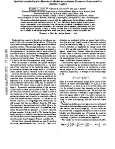
x Figure 3. The numerically determined scaling function for the 2D anisotropic system for different anisotropic constants t, different energies E and disorder W . The solid line through the data is the 2D isotropic scaling function. The y-axis is ξj λi (Mj )/ξi Mj , while the x-axis is Mj /ξj . The indices i and j may represent either the parallel or the perpendicular direction, respectively.

266

C M Soukoulis and E N Economou

Conductance G

10- 4

W=3.6 Mx10M 10MxM

10- 6 10- 8 10-10 10-12

4

8

12

16

20

24

28

32

36

M Figure 4. The conductance G in units of e2 / h of an anisotropic system M × N versus M for t = 0.1 and E = 0. Notice that G along the two directions is exactly the same. The circles and triangles plot the propagation along the short and long directions, respectively.

properly scaled with the localization lengths in the two directions, ξk and ξ⊥ . The solid line through the data in figure 3 is the 2D isotropic scaling function. This is a direct confirmation of the scaling relation, equation (15). An important consequence of equation (15) is that at the critical point, if any, the geometric mean of the ratio of the finite-size localization length to the cross section width is a constant. This was indeed found [7] to be true but interpreted instead as a result of possible conformal invariance. We point out that at the critical point, the geometric mean of the conductances along the different directions may not be a constant. This behaviour of the conductances is different from that of λM /M and needs further study for its complete understanding. To further test the scaling idea, the conductance G in the two different directions for an anisotropic system has been calculated [38]. The multichannel Landauer formula [16], G = (e2 / h) Tr(t † t), where t is the transmission matrix, has been used. With anisotropic hoppings, one should choose a geometry other than the square, such that the conductance is the same in all the directions, and then scale up the size of the system [37]. The conductance should remain isotropic if one-parameter scaling theory is correct [35]. This idea has been tested in a 2D system with t = 0.1. The ratio of the two localization lengths was found to be 10 at W = 3.6. The system of a rectangle of size M × N has been scaled up by a factor of four and, from figure 4, one can clearly see that although the conductance becomes extremely small it remains isotropic, in agreement with the predictions of the one-parameter scaling theory [4, 35]. For a square geometry and with the same parameters as in figure 4, the conductances in the two directions would diverge rapidly as the system size scales up. An extensive numerical study [38] of the scaling properties of highly anisotropic systems was performed. Scaling functions of isotropic systems are recovered once the dimension of the system in each direction is chosen to be proportional to the localization length. In the localized regime, the ratio of the localization lengths is proportional to the square root of the ratio of the conductivities which, in turn, is proportional to the strength of the anisotropy t (i.e. ξ⊥ /ξk ∼ t). Recall that in the extended regime [4, 7] the ratio of the correlation lengths is proportional to the ratio of the conductivities (i.e. ξ⊥ /ξk = σ0⊥ /σ0k ∼ 1/t 2 ). It was also shown that the geometric mean of the localization lengths is a function of the geometric mean of the conductivities. Finally, it was shown numerically that the conductances along the two different directions of the anisotropic system are the same, provided that the dimensions of the anisotropic system are proportional to the localization lengths in the corresponding directions. This procedure can be easily used in other anisotropic systems.

Electronic localization in disordered systems

267

2.11. Metal–insulator transition in 2D disordered systems As we have discussed above, the scaling theory of localization predicts that all the states are localized in a disordered 2D system. Thus, for the last two years it was generally believed that 2D disordered systems, in the absence of a magnetic field, do not undergo a metal-toinsulator transition, even at 0 K. Experiments [39] performed some considerable time ago in the 1980s generally confirmed the predictions of the scaling theory. However, in a series of recent experiments Kravchenko et al [8] reported evidence for a metal-to-insulator transition in a 2D electron gas in zero magnetic field. The new ingredient in these recent experiments [8] on MOSFETs is the much higher electron mobilities than in the experiments in the 1980s. The experimental reports for the 2D metal-to-insulator transition have created a lot of excitement in the community and both theorists and experimentalists are working hard to understand this new unexpected behaviour of a 2D strongly interacting disordered system. Although the scaling theory of localization has had great success over the last two decades, it now appears that electron–electron interactions must play a very important role in 2D systems. We feel that this is one of the most interesting and challenging problems in the field of electronic disordered systems. 3. Summary In this article we have reviewed some of the recent developments in the theory of non-interacting electrons in disordered systems. Particular emphasis has been placed on the discussion of the universal features of the electronic density of states in disordered systems. An exponential behaviour of the DOS is exhibited over many decades. The role of the disorder is, first, to shift the band edge by an amount proportional to w2 , which is given by second-order perturbation theory or by the CPA. Once the energies are measured relative to the CPA band edge, all the physical quantities of interest, including DOS, are quasi-universal, provided that the length and energy, scaled relative to disorder-dependent units of energy and length, are small. Next, the weak-interaction regime or the interference effects of the localization theory were presented. The interference between a closed Feynman path and its time-reversed path gives the unexpected result that d = 2 is the marginal dimension for localization. Another dramatic effect of the weak localization in disordered electronic systems occurs when a magnetic field is applied, in which case the theory predicts a negative magnetoresistance. Then, the scaling theory of localization, the self-consistent theory of localization and the equivalence of localization in a random potential to the existence of a bound state in a potential well were briefly presented. The potential-well analogy (PWA) facilitates explicit calculations of the localization lengths, conductivities, mobility edges, etc, from quantities that can be obtained from meanfield theories, such as the CPA. It was shown that the PWA coupled with the CPA is capable of producing results not only in qualitative agreement but also in quantitative agreement with an independent numerical approach. The advantage of the PWA–CPA approach over numerical approaches is that it is analytical and gives results relatively easily, even for complicated quantities. The PWA method was applied to 3D systems by modelling the disorder using a Gaussian, a rectangular, and a binary distribution for the random site energies. The numerical results for the DOS exhibit the quasi-universality expected from the analytical arguments (white-noise model). However, the trajectory in the energy-disorder plane of the mobility edge depends on the type of probability used. It is also discussed that the electronic wavefunctions in disordered systems are very complicated quantities. Explicit calculations have shown that the wavefunctions have strong amplitude fluctuations of various spatial extents. In particular, exactly at the mobility edge the wavefunctions can be characterized by fractal dimensionalities

268

C M Soukoulis and E N Economou

and in this sense they are fractal objects for all length scales, while they are fractal-like for lengths up to the localization (correlation) length for localized (extended) states, respectively. What we learned about the wave nature of electrons in disordered systems should enhance our understanding of the propagation of classical waves. Finally, a few remarks are included about the metal-to-insulator transition in strongly interacting systems. Acknowledgments Ames Laboratory is operated for the US Department of Energy by Iowa State University under Contract No W-7405-Eng-82. This work was supported by the Scalable Computing Laboratory of Ames Laboratory, the director for Energy Research, Office of Basic Energy Sciences, NATO Grant No CRG 940647. This work was also supported in part by EU grants and 5ENE1 Research Grants from the Greek Secretariat of Science and Technology. References [1] [2] [3] [4] [5] [6] [7]

[8] [9] [10] [11] [12]

[13] [14] [15] [16] [17] [18] [19] [20]

[21] [22] [23] [24]

Anderson P W 1958 Phys. Rev. 109 1492 Lee P A and Ramakrishnan T V 1985 Rev. Mod. Phys. 57 287 Kramer B and Mackinnon A 1993 Rep. Prog. Phys. 56 1469 Vollhardt D and W¨olfle P 1992 Electronic Phase Transitions ed W Hanke and Yu V Kopaev (New York: Elsevier) ch 1, p 38 Soukoulis C M and Economou E N 1984 Phys. Rev. Lett. 52 565 Soukoulis C M, Wang X, Li Q and Sigalas M 1999 Phys. Rev. Lett. 82 668 Li Q, Soukoulis C M, Economou E N and Grest G S 1989 Phys. Rev. B 40 2825 Zambetaki I, Li Q, Economou E N and Soukoulis C M 1996 Phys. Rev. Lett. 76 3614 Zambetaki I, Li Q, Economou E N and Soukoulis C M 1997 Phys. Rev. B 56 12 221 Kravchenko S V, Simonian D, Sarachik M P, Mason W and Furneaux J E 1996 Phys. Rev. Lett. 77 4938 Simonian D, Kravchenko S V and Sarachik M P 1996 Phys. Rev. Lett. 79 2304 Mott N F and Davis E A 1979 Electronic Processes in Non-Crystalline Materials (Oxford: Oxford University Press) Urbach F 1953 Phys. Rev. 92 1324 Cody G D 1984 Semiconductors and Semimetals vol 21B, ed B J Pankove (New York: Academic) p 11 Economou E N, Soukoulis C M, Cohen M H and Zdetsis A D 1985 Phys. Rev. B 31 6172 Cohen M H, Economou E N and Soukoulis C M 1985 Phys. Rev. B 32 8268 Cohen M H, Soukoulis C M and Economou E N 1985 Physics of Disordered Materials ed D Adler et al (New York: Plenum) p 305 Economou E N 1983 Green’s Functions in Quantum Physics 2nd edn (Heidelberg: Springer) John S, Chou M Y, Cohen M H and Soukoulis C M 1988 Phys. Rev. B 37 6963 John S, Soukoulis C M, Cohen M H and Economou E N 1986 Phys. Rev. Lett. 57 1777 Landauer R 1957 IBM J. Res. Dev. 1 223 Economou E N and Soukoulis C M 1981 Phys. Rev. Lett. 46 618 Fisher D S and Lee P A 1981 Phys. Rev. B 23 685 Thouless D 1981 Phys. Rev. Lett. 47 972 Economou E N and Soukoulis C M 1981 Phys. Rev. Lett. 47 973 Stone A D and Szafer A 1988 IBM J. Res. Dev. 32 384 Landauer R 1981 Phys. Lett. A 85 91 Kramer B and Schon G (ed) Anderson transition and mesoscopic fluctuations Physica A 167 1–314 Sokoloff J B 1985 Phys. Rep. 126 189 Soukoulis C M and Economou E N 1982 Phys. Rev. Lett. 48 1043 Zdetsis A D, Soukoulis C M and Economou E N 1986 Phys. Rev. B 33 4936 Thouless D J 1974 Phys. Rep. 13 93 Abrahams E, Anderson P W, Licciardello D C and Ramakrishan T V 1979 Phys. Rev. Lett. 42 673 Kaveh M and Mott N F 1987 Phil. Mag. 55 9 Economou E N and Soukoulis C M 1983 Phys. Rev. B 28 1093 Economou E N and Soukoulis C M 1984 Phys. Rev. B 30 1686

Electronic localization in disordered systems Zdetsis A D, Soukoulis C M, Economou E N and Grest G S 1985 Phys. Rev. B 32 7811 [25] Soukoulis C M, Zdetsis A D and Economou E N 1986 Phys. Rev. B 34 2253 [26] Soukoulis C M, Economou E N and Grest G S 1987 Phys. Rev. B 36 8649 Soukoulis C M and Grest G S 1991 Phys. Rev. B 44 4685 Soukoulis C M, Li Q and Grest G S 1992 Phys. Rev. B 45 7724 [27] Soukoulis C M and Economou E N 1981 Phys. Rev. B 24 5698 Soukoulis C M, Webman I, Grest G S and Economou E N 1982 Phys. Rev. B 26 1838 Li Q, Soukoulis C M and Economou E N 1988 Phys. Rev. B 37 8289 [28] Li Q, Soukoulis C M and Grest G S 1990 Phys. Rev. B 41 11 713 [29] Soukoulis C M, Economou E N, Grest G S and Cohen M H 1989 Phys. Rev. Lett. 62 575 Soukoulis C M, Datta S and Economou E N 1994 Phys. Rev. B 49 3800 [30] MacKinnon A and Kramer B 1981 Phys. Rev. Lett. 47 1546 [31] Economou E N, Soukoulis C M and Zdetsis A D 1985 Phys. Rev. B 31 6483 [32] Zharekeshev I K and Kramer B 1997 Phys. Rev. Lett. 79 717 and references therein [33] Cohen M H, Economou E N and Soukoulis C M 1983 Phys. Rev. Lett. 51 1202 [34] Huckestein B 1995 Rev. Mod. Phys. 67 357 and references therein [35] W¨olfle P and Bhatt R N 1984 Phys. Rev. B 30 3542 Bhatt R N, W¨olfle P and Ramakrishnan T V 1985 Phys. Rev. B 32 569 [36] Xue W, Sheng P, Chu Q J and Zhang Z Q 1989 Phys. Rev. Lett. 63 2837 Xue W, Sheng P, Chu Q J and Zhang Z Q 1990 Phys. Rev. B 42 4613 Chu Q J and Zhang Z Q 1993 Phys. Rev. B 48 10 761 [37] Apel W and Rice T M 1983 J. Phys. C: Solid State Phys. 16 L1151 [38] Li Q, Katsoprinakis S, Economou E N and Soukoulis C M 1997 Phys. Rev. B 56 R4297 [39] Bergmann G 1984 Phys. Rep. 107 1

269