Nov 24, 2009 - *Presented by S. Warzel at the XVI International Congress of Mathematical Physics, Prague 2009. 1. arXiv:0909.5432v2 [math-ph] 24 Nov 2009 ...
arXiv:0909.5432v2 [math-ph] 24 Nov 2009
Complete Dynamical Localization in Disordered Quantum Multi-Particle Systems∗ Michael Aizenman(a) and Simone Warzel(b) (a)
Departments of Physics and Mathematics Princeton University, Princeton NJ 08544, USA (b)
Zentrum Mathematik, TU M¨unchen Boltzmannstr. 3, 85747 Garching, Germany September 29, 2009
Abstract We present some recent results concerning the persistence of dynamical localization for disordered systems of n particles under weak interactions.
1
Introduction
After more than half a century, Anderson localization continues to attract the interest of a broad spectrum of researchers ranging from experimentalists, who finds its effects in systems of cold atoms and in photonic crystals [7], to mathematical physicists. Considerable progress was made in the rigorous methods for the study of the localization effects of disorder in the context of the one-particle theory [17, 14, 6]. More recently attention has centered on the role of interactions, and questions related to the persistence of the localization picture in the presence of inter-particle interactions. We shall report here on some progress which was made in that area.
1.1
The one-particle theory
The discussion of weakly interacting particles often starts from the approximation in which the interactions are ignored. That is, one first considers systems of Fermions, or Bosons possibly with on-site repulsion, subject to a fixed potential which includes random terms. Such system can be understood in terms of the one-particle theory. ∗ Presented
by S. Warzel at the XVI International Congress of Mathematical Physics, Prague 2009.
1
For particles moving on a lattice Zd , the single-particle Hamiltonian may take the form H (1) (ω) := −∆ + λ V (x; ω) , in `2 (Zd ), (1.1) where −∆ is the lattice Laplacian and the random potential incorporates a disorder parameter λ ≥ 0. For the convenience of presentation, all mathematical statements in this note are made under the assumption that the random potential V (x; ω) takes independent and indentically distributed values on the lattice sites x ∈ Zd , with a distribution P(Vx ∈ dv) = %(v) dv of a bounded, compactly supported density. When talking about localization for operators such as H (1) (ω), different notions have been used and established: Spectral localization in an energy regime I ⊂ R, refers to the statement that within the specified energy regime H (1) (ω) has only pure point spectrum, with exponentially localized eigenfunctions, cf. [17] and references therein. Dynamical localization in I ⊂ R, refers to the statement that any initially localized state, which is a wave packet with energies in I ⊂ R, will remain exponentially localized indefinitely under the time evolution. A convenient sufficient condition is that for some A, ξ ∈ (0, ∞) (both depending on I, λ), � � 2 (1) (DL) E sup hδy , e−itH PI (H (1) ) δx i ≤ A e−|x−y|/ξ t∈R
where δx ∈ `2 (Zd ) is the δ state at x and PI (H (1) ) is a spectral projection. While spectral localization provides some coarse information on the quantum time evolution via the RAGE theorem, dynamical localization in the sense of (DL) is a somewhat stronger notion. Historically, spectral localization was the first to be rigorously established by building, for d > 1 at extreme energies or large disorder, on the multiscale analysis of Fr¨ohlich and Spencer [12]; cf. [17, 14]. The first proof of dynamical localization [2] relied on the fractional moment analysis of [1]. It is one of the features of the single particle model (1.1) that in any dimension there is an extreme disorder regime, with λ exceeding some finite λ1 , in which one has complete dynamical localization, meaning that all states are localized and dynamical localization (DL) holds with I = R. For the single particle model (1.1) in d = 1 complete dynamical localization with critical disorder strength λ1 = 0 was established already in [15]. For higher dimensions, d ≥ 1, an explicit bound on λ1 can be found in [2].
1.2
The influence of interaction on localization: a challenge
It is not hard to see that the above localization properties are inherited by a system of non-interacting particles with a one-particle Hamiltonian corresponding to (1.1). An important question however, is whether such behavior will persist under the addition of interparticle interactions. Especially interesting is the situation where there are n fermions in a region of volume |Λ|, with |Λ| → ∞ and n/|Λ| → ρ > 0.
2
A rather strong claim is being advocated by Basko, Aleiner and Altshuler [8], who argue that under strong disorder weak interactions do not change the qualitative picture of localization as it is seen in the non-interacting model. The proposal is rather startling. It includes the claim that if the system of particles of an overall positive density is started at a initial state at which the distribution in space of particles and energy is far from uniform, its irregularity will persist indefinitely under the time evolution. This seems to run against the vague equidistribution principle, by which one expects that except under unusual circumstances, such as in the noninteracting integrable model, the initial state will evolve in time (in a weak enough sense) towards states which maximize the entropy, in a coarse-grained sense, subject to the given energy and particle number constraints. Persistence of localization is not undisputed among physicist. In particular, longrange repulsive interactions are conjectured to have a delocalizing effect [16]. Rigorous methods are still far from allowing one to decide whether complete localization will persist or perish in the presence of interactions. Furthermore, the analysis of even a fixed number of particles with short range interactions in the infinite-volume limit has presented difficulties, and we will report on some recent progress [10, 11, 5] made in this direction. As an side we note that the dynamics of multiparticle systems bear some relation to non-linear evolutions. Recent results on that topic are discussed in [18].
2 2.1
Dynamical localization for multi-particle systems The n-particle Hamiltonian
We will be concerned with a system of finitely many interacting particles in the random potential described above. The n-particle Hamiltonian is given by H (n) (ω) :=
n X
[−∆j + λ V (xj ; ω)] + U(x; α),
in
`2 (Zd )n
(2.1)
j=1
acting in the Hilbert space over all configurations x = (x1 , . . . , xn ) ∈ (Zd )n . Here the last term is a p-site interaction of range `U < ∞: U(x; α) :=
p X k=1
αk
X
UA ((Nu (x))u∈A ) .
d
A⊂Z :|A|=k diamA≤`U
It is described in term of an interaction parameter α = (α1 , . . . , αp ) ∈ Rp and a function UA : N|A| → R which is bounded by some n-dependent constant, kUA k ≤ cP n < ∞, and translational invariant. The latter depends on the number Nu (x) := n j=1 δu,xj of particles of the configuration x = (x1 , . . . , xn ), which are at sites u ∈ A in the pattern A ⊂ Zd . Simply stated examples which are already of interest are short range pair interactions for which p = 2 and U{u,v} (Nu (x), Nv (x)) = Nu (x)Nv (x) δ|u−v|,1 . 3
2.2
The main result
Our main result establishes the existence, for any dimension and any number of parti(p) cles, of a regime Ln in the space of basic parameters of the model, (λ, α) ∈ R+ ×Rp , for which complete dynamical localization with a uniform localization length occurs for up to n particles. The proof gives an inductive algorithm for the construction of such localization regimes, albeit at what may be a possibly far too restrictive manner. The first proof of spectral localization for two particles was presented in [11], using the multiscale approach. The result presented below was derived by different means, which allow also rather simple control of the dynamical localization. The localization regime covered by the result presented below may be best described in terms of the extreme sets it includes, namely: (p)
Strong disorder for each α ∈ Rp there is λ(α) such that the localization regime Ln includes the cone in the parameter space R+ ×Rp where the interaction strengths are dominated by α, and the disorder strength exceeds λ(α). Weak interactions for any λ > λ1 , i.e. disorder strength at which the one-particle Hamiltonian exhibits complete localization, there are αj (λ) > 0 , j = {1, ..., p}, (p) such that Ln includes all (λ, α0 ) for which |α0j | ≤ |αj (λ)| componentwise. Thus, the weak localization region includes some neighborhood of the entire localization regime (λ1 , ∞)×{0} of the n particle unperturbed system. In case d = 1, λ1 = 0, so this includes all positive values of λ. Having introduced these notions we may present the result of [5]: (p)
Theorem 2.1 ([5]). For each n, p ∈ N there is an open set Ln ⊂ R+ × Rp which includes regimes of strong disorder and weak interactions, for which at some A, ξ < ∞ (p) and all (λ, α) ∈ Ln , k ∈ {1, . . . , n}, and all x, y ∈ (Zd )k : � 2 � −itH (k) E sup hδx , e δy i ≤ A e−distH (x,y)/ξ , (2.2) t∈R
where the exponential decay is in terms of the Hausdorff pseudo-distance between the configurations x = (x1 , . . . , xk ) and y = (y1 , . . . , yk ) � � distH (x, y) := max max dist(xi , y), max dist(yi , x) (2.3) 1≤i≤k
1≤i≤k
As was mentioned, spectral localization follows from (2.2) by the Wiener criterion.
2.3
Comments on the result
Theorem 2.1 is formulated for distinguishable particles. For Fermions, or Bosons, the relevant Hilbert spaces are subspaces of the space which this theorem covers, and thus the results apply by restriction. Furthermore, hard core interactions can also be added without requiring any modification in the proof of the extended statement.
4
It is worth pointing out that for systems of n > 2 particles some subtleties show up in the decay rate seen in (2.2). A natural decay rate for systemsP with permutation n symmetry is the symmetrized distance: distS (x, y) := minπ∈Sn j=1 |xj − yπj | , where Sn is the permutation group of {1, ..., n}. In contrast, distH (x, y) is not a metric, if n > 2. The Hausdorff pseudo-distance bounds (2.2) allow for the possibility that if the initial configuration had some particles within the localization distance from each other then such ‘excess charge’ may transfer among the occupied regions. ??
Figure 1: A transition between two configurations which are close in the Hausdorff pseudodistance, but not otherwise.
One could wonder whether Theorem 2.1 does not immediately follow from the existing localization results. After all, a configuration of n particles in Zd may be regarded as a single particle in Zdn evolving under a Hamiltonian which is of the (n) (nd) form + U (x) + λ V (x; ω) with a random potential V (x; ω) = Pn H (ω) = −∆ V (x ; ω). However, the random potential V (x; ω) does not take independent j j=1 values at configurations with one coinciding particle and in this sense is of infinite range. The number of its degrees of freedom is only a fractional power ( n1 ) of the number of configuration. The technical problem which this causes is behind the above mentioned limitation of the bound (2.2).
3
Outline of the proof
The proof of Theorem 2.1 cannot be fitted in this short summary, but we may comment on the flow of the argument [5]. It consists of three steps: 1. Proof of the finiteness of fractional moments of the Green function. 2. Elucidation of the relation of a multiparticle eigenfunction correlator with the Green function’s fractional moments. 3. Inductive construction of domains of uniform localization in parameter space. The first is a sine qua non condition for the fractional moment technique for localization [1]. It is related to the celebrated Wegner estimate, which however does not play a direct role in the analysis. The proof is rather easy, as is also the case for the Wegner estimate for many-particle systems. The second step follows the strategy by which dynamical localization is established for single particles [2], for which some adjustments to the multi-particle setup are required.
5
Once the first two preparatory steps are taken, the third step constitutes the core of the argument.
3.1
Finiteness of fractional moments of the Green function
An essential tool for the analysis is the finite-volume, Λ ⊂ Zd , Green function
�−1 � (n) (n) GΛ (x, y; z) := δx , HΛ − z δy ,
(3.1)
(n)
with HΛ denoting the restriction of (2.1) to `2 (Λ)n . The first step towards exponential bounds is to prove finiteness of the fractional moments. In fact, even a conditional average makes them finite. Lemma 3.1. For any s ∈ (0, 1) there is C < ∞ such that for any Λ ⊆ Zd , any two (not necessarily distinct) sites u1 , u2 ∈ Λ and any pair of configurations x, y, which have a particle at u1 , u2 respectively, s � � C (n) E GΛ (x, y; z) {V (v)}v6∈{u1 ,u2 } ≤ |λ|s
(3.2)
for all z ∈ C, and λ 6= 0. Sketch of proof. In its dependence on V (u1 ) and V (u2 ), the Hamiltonian is of the Pn (n) form: HΛ = A+λ V (u1 ) Nu1 +λ V (u2 ) Nu2 , where (Nu ψ) (x) := k=1 δxk ,u ψ(x) stands for the number operator. The assertion is therefore implied by the weak-L1 estimate from [4]: Z h D√ i E √ C[%] −1 1 N φ, (ξ N + η M − K) M ψ > t %(ξ) %(η) dξ dη ≤ kφk kψk , t 2 R with operators N, M ≥ 0 and K dissipative. The finiteness (3.2) is the analogue of a Wegner estimate in the multi-scale method. As has been noticed in [9, 13], it follows similar to the one-particle case from the monotonicity used in the above proof.
3.2
Eigenfunction correlator and its relation to Green function (n)
For the finite-volume Hamiltonian HΛ , we define the eigenfunction correlator, associated with an energy regime I ⊂ R, as the sum X (n) (n) QΛ (x, y; I) := (3.3) hδx , P{E} (HΛ ) δy i , (n)
E∈σ(HΛ )∩I
where P{E} is a spectral projection. Ignoring some subtleties related to the passage to the infinite-volume limit Λ ↑ Zd (which are discussed in detail in [2, 5]), the elementary (n) (n) bound hδx , e−itHΛ ) δy i ≤ QΛ (x, y; R) shows that the eigenfunction correlator is 6
an important tool for establishing dynamical localization [15, 2]. The following key lemma states the equivalence of exponential decay in the Hausdorff pseudo-distance (though not in the symmetric distance) of the eigenfunction correlator and of the Green function’s fractional moments. Lemma 3.2. The following statements are equivalent: 1. There is A, ξ < ∞ such that for all x, y ∈ (Zd )k : h i (k) sup sup E QΛ (x, y; I) ≤ A e− distH (x,y)/ξ .
(3.4)
I⊂R Λ⊂Zd
2. There is A, ξ < ∞ and s ∈ (0, 1) such that for all x, y ∈ (Zd )k : Z h s i 1 (k) sup sup E GΛ (x, y; E) dE ≤ A e− distH (x,y)/ξ . |I| d I⊂R Λ⊂Z |I {z } |I|≥1
(3.5)
bI [... ] =: E
In the proof of the main result we repeatedly change horses between estimates on the kernels of G and Q. The kernel Q(x, y) is what is ultimately need, and it is also a very convenient tool for the induction step. Yet, G(x, y) has a more convenient perturbation theory. In the induction step described below one puts together two mutually non-interacting subsystems and then turns on the interaction between them. Thus, we start with the system partitioned into J, K ⊂ {1, . . . , n}, J ∩ K = ∅, and a Hamiltonian of the form (J,K) (J) (K) HΛ := HΛ ⊕ HΛ acting on `2 (Λ)|J| ⊗ `2 (Λ)|K| . Then: • The Green function of the composite system is a convolution, Z dE (K) (J) (J,K) (x, y; z) = GΛ (xJ , yJ ; z − E) GΛ (xK , yK ; E) GΛ 2πi C
(3.6)
(K)
involving a contour integral encircling the spectrum of HΛ . Moment estimates for the combined system are complicated by the unboundedness of G and possible correlations between the eigenvalues of the subsystems. • On the other hand, the eigenfunction correlator is bounded and we may use: (J,K)
QΛ
(J)
(K)
(x, y; I) ≤ QΛ (xJ , yJ ; R) QΛ (xK , yK ; R) ,
(3.7)
by which the exponential decay of the subsystems passes to the joint system.
7
3.3
Inductive construction of domains of localization in parameter space
In view of the equivalence of the exponential decay in the Hausdorff distance of the eigenfunction correlator and of the fractional moments of the Green function, it is natural to define localization regimes as follows. Definition 3.1. An open subset of the parameter space, L ⊂ R+ × Rp is said to be a domain of uniform n-particle localization if for some s ∈ (0, 1) there exists ξ < ∞ and A < ∞ such that Z h s i 1 (k) E GΛ (x, y; E) dE ≤ A e− distH (x,y)/ξ . (UL) sup sup I⊂R Λ⊂Zd |I| I |I|≥1
holds for all (λ, α) ∈ L, all k ∈ {1, ..., n}, and all x, y ∈ (Zd )k . (p)
(p)
Our aim is to inductively construct Ln starting from the domain L1 = (λ1 , ∞) ⊂ R+ of uniform one-particle localization, whose existence is guaranteed in [2] (and [15] (p) for d = 1). For the induction step we assume that Ln−1 is a domain of uniform (n−1)particle localization and proceed by distinguishing two cases: 1. Localization for non-clustered configurations. Here we deal with two configuration x, y of which at least one is of diameter (diam(x) := maxj,k |xj −xk |) comparable with their Haussdorff distance. A key lemma provides the bound: h i b I |G(n) (x, y)|s sup sup E Λ I⊂R Λ⊆Zd |I|≥1
� � �� 1 max{diam(x), diam(y)} ≤ A exp − min distH (x, y), (3.8) ξ n−1 (p)
for all (λ, α) ∈ Ln−1 , (which, strictly speaking, is only valid under the addi(p) tional assumption of Ln−1 being sub-conical, cf. [5]).
Figure 2: The solid line is the full and the dotted lines represent the Green function of the partially non-interacting system which, by assumption and due to arguments based on (3.7) decay exponentially. Due to finite range, the interaction is localized to the shaded strip of width 2`U about the diagonal.
The proof of (3.8) proceeds by breaking the configuration in two parts and removing the intercluster interaction. Standard perturbation theory then yields an expansion in U which in case n = 2, d = 1 is pictorially explained in configuration space in Fig 2. 8
The bound (3.8) is rather crude in its dependence on the particle number. It is the main reason why our bounds on the localzation length degrade rapidly with n. (ii) Localization for clustered configurations. This refers to configurations with diameter less than half their separation. The issue which is to be addressed is the possible formation of a quasi-particle which is not constrained by previous localization bounds. A convenient quantity to monitor is Bs(n) (L) := sup sup |∂ΛL | I⊂R Ω⊆ΛL |I|≥1
X
X
s i h b I G(n) (x, y) , E Ω
(3.9)
y∈∂ΛL x∈C (n) (Ω;0) L (n)
y∈CL (Ω;y) (n)
where CL (Λ; x) denotes the collection of configurations of diameter less than L/2 and at least one particle at x. • one has at least one particle at 0, and • the other one has at least one particle at the boundary ∂ΛL of the box; cf. illustration in real space.
Localization bounds for clustered configurations proceed through rescaling inequal(n) ities for Bs (L). The key statement is: Lemma 3.3. There exists s ∈ (0, 1), a, A, p < ∞, and ν > 0 such that Bs(n) (2L) ≤
a B (n) (L)2 + A L2p e−2νL |λ|s s
(3.10)
(p)
for all (λ, α) ∈ Ln−1 , (which is again assumed to be sub-conical, cf. [5]). Part of the proof of this lemma resembles the proof of finite-volume criterial for one particle localization in [3]. In view of the infinite-range correlations of the random potential in configuration space discussed at the beginning of this section, a crucial observation is the following. When placing two boxes of length L/2 about configurations x and y in the above picture, the random variables associated with those boxes are independent due to the spatial separation. Moreover, the error when restricting the sum (n) in the definition of Bs (2L) to configurations x, y which have a diameter less than L/4 can be controlled by (3.8) yielding the second term on the right side in (3.10). It is not hard to see that rescaling inequalities such as (3.10) imply exponential (n) decay provided the quantity |λ|a s Bs (L) is small on some scale L. This is the require(p)
ment which determines Ln . Namely,
9
• in case of strong disorder and arbitrary value of the interaction α we choose L fixed and λ small enough. • in case of weak interaction and arbitrary value of the disorder λ > λ1 we appeal (n) to [1, 3] which imply that Bs (L) → 0 as L → ∞ for α = 0. Since the (n) finite-volume quantity Bs (L) is continuous in some neighborhood of α = 0 we choose L and α accordingly.
4
Some remaining challenges
While Theorem 2.1 is formulated for interactions of finite range, its proof allows for extension to interactions of with exponential falloff. However, it it does not address questions about the effects of Coulomb interactions. An important outstanding challenge it to resolve the question which is commented upon in Section 2.3: does localization persists (with uniform bounds) even for large systems at a positive density of particles?
Acknowledgments This work was partially supported by the National Science Foundation under grants DMS-0602360 (MA), DMS-0701181 (SW) and a Sloan Fellowship (SW).
References [1] M. Aizenman and S. Molchanov, Localization at large disorder and at extreme energies: an elementary derivation, Comm. Math. Phys., 157 245–278 (1993). [2] M. Aizenman, Localization at weak disorder: some elementary bounds, Rev. Math. Phys. 6, 1163-1182 (1994). [3] M. Aizenman, J. H. Schenker, R. M. Friedrich, and D. Hundertmark, Finitevolume criteria for Anderson localization. Comm. Math. Phys. 224 219–253 (2001). [4] M. Aizenman, A. Elgart, S. Naboko, J. H. Schenker, and G. Stolz, Moment analysis for localization in random Schr¨odinger operators, Invent. Math. 163, 343-413 (2006). [5] M. Aizenman and S. Warzel, Localization Bounds for Multiparticle Systems, Commun. Math. Phys. 293, 903-934 (2009). [6] M. Aizenman and S. Warzel, Random Schr¨odinger Operators, Lecture Notes, in preparation. [7] A. Aspect and M. Inguscio, Anderson localization of ultracold atoms, Phys. Today August 2009. 10
[8] D. M. Basko, I. L. Aleiner, and B. L. Altshuler, Metal-insulator transition in a weakly interacting many-electron system with localized single-particle states, Annals of Physics 321 1126-1205 (2006). [9] V. Chulaevsky, and Y. M. Suhov, Wegner bounds for a two-particle tight binding model, Comm. Math. Phys. 283, 479-489 (2008). [10] V. Chulaevsky, and Y. M. Suhov, Eigenfunctions in a two-particle Anderson tight binding model, Comm. Math. Phys. 289, 701-723 (2009). [11] V. Chulaevsky and Y. Suhov, Multi-particle Anderson localisation: Induction on the number of particles, Math. Phys. Anal. Geom. 12, 117-139 (2009). [12] J. Fr¨ohlich and T. Spencer, Absence of diffusion in the Anderson tight binding model for large disorder or low energy, Comm. Math. Phys. 88, 151–184 (1983). [13] W. Kirsch, A Wegner estimate for multi-particle random Hamiltonians, J. Math. Phys. Anal. Geom. 4, 121–127 (2008). [14] W. Kirsch, An invitation to random Schr¨odinger operators (with appendix by F. Klopp). pp. 1-119 in: Random Schr¨odinger Operators. M. Disertori, W. Kirsch, A. Klein, F. Klopp, V. Rivasseau, Panoramas et Synth`eses 25 (2008). [15] H. Kunz and B. Souillard, Sur le spectre des op´erateurs aux diff´erences finies al´eatoires, Commun. Math. Phys. 78, 201-246 (1980). [16] D. L. Shepelyansky, Three-dimensional Anderson transition for two electrons in two dimensions, Phys. Rev. B, 61 4588 - 4591 (2000). [17] P. Stollmann, Caught by disorder: bound states in random media, (Birkh¨auser, 2001). [18] W.-M. Wang and Z. Zhang, Long time Anderson localization for the nonlinear random Schr¨odinger equation, J. Stat. Phys., 134, 953-968 (2009).
11