Section 2.8: Key Results from Nonlinear Programming Sensitivity. Analysis. ... ble descent algorithm for convex mathematical programs with a differentiable.
2 Elements of Nonlinear Programming
T
he primary intent of this chapter is to introduce the reader to the theoretical foundations of nonlinear programming. Particularly important are the notions of local and global optimality in mathematical programming, the Kuhn-Tucker necessary conditions for optimality in nonlinear programming, and the role played by convexity in making necessary conditions sufficient. The following is an outline of the principal topics covered in this chapter:
Section 2.1: Nonlinear Program Defined. A formal definition of a finitedimensional nonlinear mathematical program, with a single criterion and both equality and inequality constraints, is given. Section 2.2: Other Types of Mathematical Programs. Definitions of linear, integer and mixed integer mathematical programs are provided. Section 2.3: Necessary Conditions for an Unconstrained Minimum. We derive necessary conditions for a minimum of a twice continuously differentiable function when there are no constraints. Section 2.4: Necessary Conditions for a Constrained Minimum. Relying on geometric reasoning, the Kuhn-Tucker conditions, as well as the notion of a constraint qualification, are introduced. Section 2.5: Formal Derivation of the Kuhn-Tucker Conditions. A formal derivation of the Kuhn-Tucker necessary conditions, employing a conic definition of optimality and theorems of the alternative, is provided. Section 2.6: Sufficiency, Convexity, and Uniqueness. We provide formal definitions of a convex set and a convex function. Then we show formally how those notions influence sufficiency and uniqueness of a global minimum. Section 2.8: Key Results from Nonlinear Programming Sensitivity Analysis. We provide a succinct review of nonlinear programming sensitivity analysis. © Springer Science+Business Media New York 2016 T.L. Friesz, D. Bernstein, Foundations of Network Optimization and Games, Complex Networks and Dynamic Systems 3, DOI 10.1007/978-1-4899-7594-2_2
23
24
2. Elements of Nonlinear Programming
Section 2.9: Numerical and Graphical Examples. We provide graphical and numerical examples that illustrate the abstract optimality conditions introduced in previous sections of this chapter. Section 2.10: One-Dimensional Optimization. We provide a brief discussion of numerical techniques (sometimes called line-search methods) for solving one-dimensional minimization problems. Section 2.11: Descent Algorithms in �n . We consider a generic feasible descent algorithm for convex mathematical programs with a differentiable objective function and differentiable constraints.
2.1
Nonlinear Program Defined
We are presently interested in a type of optimization problem known as a finite-dimensional mathematical program, namely: find a vector x ∈ �n that satisfies ⎫ min f (x)⎪ ⎪ ⎪ ⎬ subject to h(x) = 0 (2.1) ⎪ ⎪ ⎪ ⎭ g(x) ≤ 0 where x = (x1 , . . . , xn )T ∈ �n f (·) : �n −→ �1 g(x) = (g1 (x), . . . , gm (x))T : �n −→ �m h(x) = (h1 (x), . . . , hq (x))T :
�n −→ �q
We call the xi for i ∈ {1, 2, . . . , n} decision variables, f (x) the objective function, h(x) = 0 the equality constraints and g(x) ≤ 0 the inequality constraints. Because the objective and constraint functions will in general be nonlinear, we shall consider (2.1) to be our canonical form of a nonlinear mathematical program (NLP). The feasible region for (2.1) is X ≡ {x : g(x) ≤ 0, h(x) = 0} ⊂ �n
(2.2)
which allows us to state (2.1) in the form ⎫ min f (x)⎬ subject to
x ∈ X⎭
The pertinent definitions of optimality for the NLP defined above are:
(2.3)
25
2.2. Other Types of Mathematical Programs
Definition 2.1 (Global minimum) Suppose x∗ ∈ X and f (x∗ ) ≤ f (x) for all x ∈ X. Then f (x) achieves a global minimum on X at x∗ , and we say x∗ is a global minimizer of f (x) on X. Definition 2.2 (Local minimum) Suppose x∗ ∈ X and there exists an � > 0 such that f (x∗ ) ≤ f (x) for all x ∈ [N� (x∗ ) ∩ X], where N� (x∗ ) is a ball of radius � > 0 centered at x∗ . Then f (x) achieves a local minimum on X at x∗ , and we say x∗ is a local minimizer of f (x). In practice, we will often relax the formal terminology of Definitions 2.1 and 2.2 and refer to x∗ as a global minimum or a local minimum, respectively.
2.2
Other Types of Mathematical Programs
We note that the general form of a continuous mathematical program (MP) may be specialized to create various types of mathematical programs that have been studied in depth. In particular, if the objective function and all constraint functions are linear, (2.1) is called a linear program (LP). In such cases, we normally add slack or surplus variables to the inequality constraints to convert them into equality constraints. That is, if we have the constraint gi (x) ≤ 0
(2.4)
gi (x) + si = 0
(2.5)
we convert it into
and solve for both x and si . The variable si is called a slack variable and obeys si ≥ 0
(2.6)
If we have an inequality constraint of the form gj (x) ≥ 0
(2.7)
gj (x) − sj = 0
(2.8)
sj ≥ 0
(2.9)
we convert it to the form
where
is called a surplus variable. Thus, we can convert any problem with inequality constraints into one that has only equality constraints and non-negativity restrictions. So without loss of generality, we take the canonical form of the linear programming problem to be
26
2. Elements of Nonlinear Programming
min
n �
ci xi
i=1
subject to n �
aij xj = bi
i = 1, . . . , m
Uj ≥xj ≥ Lj
j = 1, . . . , n
j=1
x ∈ �n
⎫ ⎪ ⎪ ⎪ ⎪ ⎪ ⎪ ⎪ ⎪ ⎪ ⎪ ⎪ ⎪ ⎪ ⎬ ⎪ ⎪ ⎪ ⎪ ⎪ ⎪ ⎪ ⎪ ⎪ ⎪ ⎪ ⎪ ⎪ ⎭
(2.10)
where n > m. This problem can be restated further, using matrix and vector notation, as ⎫ min cT x ⎪ ⎪ ⎪ ⎪ ⎪ ⎪ ⎬ Ax = b ⎪
subject to
⎪ U ≥x ≥ L⎪ ⎪ ⎪ ⎪ ⎪ ⎪ n⎭ x∈�
LP
(2.11)
where c ∈ �n , b ∈ �n , and A ∈ �m×n . If the objective function and/or some of the constraints are nonlinear, (2.1) is called a nonlinear program (NLP) and is written as:
gi (x) ≤ 0
⎫ ⎪ ⎪ ⎪ ⎪ ⎪ ⎪ ⎬ i = 1, . . . , m ⎪
hi (x) = 0
i = 1, . . . , q
min f (x) subject to
x ∈ �n
⎪ ⎪ ⎪ ⎪ ⎪ ⎪ ⎪ ⎭
NLP
(2.12)
If all of the elements of x are restricted to be a subset of the integers and I n denotes the integer numbers, the resulting program min f (x) subject to
gi (x) ≤ 0
i = 1, . . . , m
hi (x) = 0
i = 1, . . . , q
x ∈ In
⎫ ⎪ ⎪ ⎪ ⎪ ⎪ ⎪ ⎪ ⎬ ⎪ ⎪ ⎪ ⎪ ⎪ ⎪ ⎪ ⎭
IP
(2.13)
is called an integer program (IP). If there are two classes of variables, some that are continuous and some that are integer, as in
27
2.3. Necessary Conditions for an Unconstrained Minimum
gi (x, y) ≤ 0
⎫ ⎪ ⎪ ⎪ ⎪ ⎪ ⎪ ⎬ i = 1, . . . , m ⎪
hi (x, y) = 0
i = 1, . . . , q
min f (x, y) subject to
x ∈ �n
y ∈ In
⎪ ⎪ ⎪ ⎪ ⎪ ⎪ ⎪ ⎭
MIP
(2.14)
the problem is known as a mixed integer program (MIP).
2.3
Necessary Conditions for an Unconstrained Minimum
Necessary conditions for optimality in the mathematical program (2.1) are systems of equalities and inequalities that must hold at an optimal solution x∗ ∈ X. Any such condition has the logical structure: If x∗ is optimal, then some property P(x∗ ) is true. Necessary conditions play a central role in the analysis of most mathematical programming models and algorithms. We begin our discussion of necessary conditions for mathematical programs by considering the general finite-dimensional mathematical program introduced in the previous section. In particular, we want to state and prove the following result for mathematical programs without constraints: Theorem 2.1 (Necessary conditions for an unconstrained minimum) Suppose f : �n −→ �1 is twice continuously differentiable for all x ∈ �n . Then necessary conditions for x∗ ∈ �n to be a local or global minimum of min f (x) subject to x ∈ �n are ∇f (x∗ ) ∇2 f (x∗ )
= 0 � 2 � ∂ f (x∗ ) ≡ must be positive semidefinite ∂xi ∂xj
(2.15) (2.16)
That is, the gradient must vanish and the Hessian must be a positive semidefinite matrix at the minimum of interest. Proof. Since f (.) is twice continuously differentiable, we may make a Taylor series expansion in the vicinity of x∗ ∈ �n , a local minimum: f (x)
=
T
f (x∗ ) + [∇f (x∗ )] (x − x∗ ) + 2
+ �x − x∗ � O (x − x∗ )
1 T (x − x∗ ) ∇2 f (x∗ ) (x − x∗ ) 2
28
2. Elements of Nonlinear Programming
where O (x − x∗ ) −→ 0 as x −→ x∗ . If ∇f (x∗ ) = 0, then by picking x = x∗ − θ∇f (x∗ ) we can make f (x) < f (x∗ ) for sufficiently small θ > 0 thereby directly contradicting the fact that x∗ is a local minimum. It follows that condition (2.15) is necessary, and we may write f (x) = f (x∗ ) +
1 T 2 (x − x∗ ) ∇2 f (x∗ ) (x − x∗ ) + �x − x∗ � O (x − x∗ ) 2
If the matrix ∇2 f (x∗ ) is not positive semidefinite, there must exist a direction vector d ∈ �n such that d = 0 and dT ∇2 f (x∗ ) d < 0. If we now choose x = x∗ +θd, it is possible for sufficiently small θ > 0 to realize f (x) < f (x∗ ) in direct contradiction of the fact that x∗ is a local minimum.
2.4
Necessary Conditions for a Constrained Minimum
We comment that necessary conditions for constrained programs have the same logical structure as necessary conditions for unconstrained programs introduced in Sect. 2.3; namely: If x∗ is optimal, then some property P(x∗ ) is true. For constrained programs obeying certain regularity conditions, we will shortly find that P(x∗ ) is either the so-called Fritz John conditions or the Kuhn-Tucker conditions. We now turn to the task of providing an informal motivation of the Fritz John conditions, which are the pertinent necessary conditions for the case when no constraint qualification is imposed.
2.4.1
The Fritz John Conditions
A fundamental theorem on necessary conditions is: Theorem 2.2 (Fritz John conditions) Let x∗ be a (global or local) minimum of ⎫ ⎬ min f (x) (2.17) subject to x ∈ F = {x ∈ X0 : g(x) ≤ 0, h(x) = 0} ⊂ �n ⎭ where X0 is a nonempty open set in �n , g : �n −→ �m , and h : �n −→ �q . Assume that f (x), gi (x) for i ∈ [1, m] and hi (x) for i ∈ [1, q] have continuous first derivatives everywhere on F . Then there must exist multipliers μ0 ∈ �1+ , T q μ = (μ1 , . . . , μm )T ∈ �m + , and λ = (λi , . . . ; λq ) ∈ � such that μ0 ∇f (x∗ ) +
m �
μi ∇gi (x∗ ) +
i=1
μi gi (x∗ ) = 0
q �
λi ∇hi (x∗ ) = 0
(2.18)
i=1
∀ i ∈ [1, m]
(2.19)
29
2.4. Necessary Conditions for a Constrained Minimum μi ≥ 0
∀ i ∈ [0, m]
(μ0 , μ, λ) = 0 ∈ �
m+q+1
(2.20) (2.21)
Conditions (2.18)–(2.21) together with h(x) = 0 and g(x) ≤ 0 are called the Fritz John conditions. We will give a formal proof of their validity in Sect. 2.5.3. For now our focus is on how the Fritz John conditions are related to the KuhnTucker conditions, which are the chief applied notion of a necessary condition for optimality in mathematical programming.
2.4.2
Geometry of the Kuhn-Tucker Conditions
Under certain regularity conditions called constraint qualifications, we may be certain that μ0 = 0. In that case, without loss of generality, we may take μ0 = 1. When μ0 = 1, the Fritz John conditions are called the KuhnTucker conditions and (2.18) is called the Kuhn-Tucker identity. In either case, (2.19) and (2.20) together are called the complementary slackness conditions. Sometimes it is convenient to define the Lagrangean function: L(x,λ, μ0 , μ) ≡ μ0 f (x) + λT h(x) + μT g(x)
(2.22)
By virtue of this definition, identity (2.18) can be expressed as ∇x L(x∗ , λ, μ0 , μ) = 0
(2.23)
At the same time (2.19) and (2.20) can be written as μT g(x∗ ) = 0
(2.24)
μ≥0
(2.25)
Furthermore, we may give a geometrical motivation for the Kuhn-Tucker conditions by considering the following abstract problem with two decision variables and two inequality constraints: ⎫ min f (x1 , x2 ) ⎪ ⎪ ⎪ ⎬ subject to g1 (x1 , x2 ) ≤ 0 (2.26) ⎪ ⎪ ⎪ ⎭ g2 (x1 , x2 ) ≤ 0 The functions f (.), g1 (.) , and g2 (.) are assumed to be such that the following are true: (1) all functions are differentiable; (2) the feasible region F ≡ {(x1 , x2 ) : g1 (x1 , x2 ) ≤ 0, g2 (x1 , x2 ) ≤ 0} is a convex set;
30
2. Elements of Nonlinear Programming
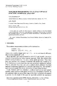
Figure 2.1: Geometry of an Optimal Solution (3) all level sets Sk ≡ {(x1 , x2 ) : f (x1 , x2 ) ≤ fk } are convex, where fk ∈ [α, +∞) ⊂ �1+ is a constant and α is the unconstrained minimum of f (x1 , x2 ); and (4) the level curves
Ck = (x1 , x2 ) : f (x1 , x2 ) = fk ∈ �1 for the ordering f0 < f1 < f2 < · · · < fk do not cross one another, and Ck is the locus of points for which the objective function has the constant value fk . Figure 2.1 is one realization of the above stipulations. Note that there is an uncountable number of level curves and level sets since fk may be any real number from the interval [α, +∞) ⊂ �1+ . In Fig. 2.1, because the gradient of any function points in the direction of maximal increase of the function, we see there is a μ1 ∈ �1++ such that ∇f (x∗1 , x∗2 ) = −μ1 ∇g1 (x∗1 , x∗2 ),
(2.27)
where (x∗1 , x∗2 ) is the optimal solution formed by the tangency of g1 (x∗1 , x∗2 ) = 0 with the level curve f (x∗1 , x∗2 ) = f3 . Evidently, this observation leads directly to ∇f (x∗1 , x∗2 ) + μ1 ∇g1 (x∗1 , x∗2 ) + μ2 ∇g2 (x∗1 , x∗2 )
= 0
(2.28)
μ1 g1 (x∗1 , x∗2 )
= 0
(2.29)
μ2 g2 (x∗1 , x∗2 )
= 0
(2.30)
μ1 , μ2
≥ 0,
(2.31)
31
2.4. Necessary Conditions for a Constrained Minimum
Note that g1 (x∗1 , x∗2 ) = 0 allows us to conclude that (2.29) holds even though μ1 > 0. Similarly, (2.27) implies that μ2 = 0, so (2.30) holds even though g2 (x∗1 , x∗2 ) = 0. Clearly, the nonnegativity conditions (2.31) also hold. By inspection, (2.28)–(2.31) are the Kuhn-Tucker conditions (Fritz John conditions with μ0 = 1) for the mathematical program (2.26).
2.4.3
The Lagrange Multiplier Rule
We wish to give a statement of a particular instance of the Kuhn-Tucker theorem on necessary conditions for mathematical programming problems, together with some informal remarks about why that theorem holds when a constraint qualification is satisfied. Since our informal motivation of the Kuhn-Tucker conditions in the next section depends on the Lagrange multiplier rule (LMR) for mathematical programs with equality constraints, we must first state and motivate the LMR. To that end, take x and y to be scalars and F (x, y) and h(x, y) to be scalar functions. Consider the following mathematical program with two decision variables and a single equality constraint: ⎫ min F (x, y)⎬ (2.32) subject to h(x, y) = 0 ⎭ Assume that h (x, y) = 0 may be manipulated to find x in terms of y. That is, we know x = H (y) (2.33) so that F (x, y) = F [H (y) , y] ≡ Φ (y)
(2.34)
and (2.32) may be thought of as the one-dimensional unconstrained problem min Φ (y) y
(2.35)
which has the apparent necessary condition dΦ (y) =0 dy
(2.36)
By the chain rule we have the alternative form dΦ (y) ∂F (H, y) ∂F (H, y) ∂H = + =0 dy ∂y ∂H ∂y
(2.37)
Applying the chain rule to the equality constraint h (x, y) = 0 leads to dh(x, y) =
∂h ∂h dx + dy = 0 ∂x ∂y
(2.38)
from which we obtain ∂x ∂h/∂y = (−1) ∂y ∂h/∂x
(2.39)
32
2. Elements of Nonlinear Programming The necessary condition (2.37), with the help of (2.33) and (2.39), becomes ∂F ∂F ∂x ∂F ∂F ∂h/∂y + = + (−1) ∂y ∂x ∂y ∂y ∂x ∂h/∂x =
∂F/∂x ∂h ∂F + (−1) ∂y ∂h/∂x ∂y
=
∂h ∂F +λ =0 ∂y ∂y
(2.40)
where we have defined the Lagrange multiplier to be λ = (−1)
∂F/∂x ∂h/∂x
(2.41)
The LMR consists of (2.40) and (2.41), which we restate as ∂F ∂h +λ ∂x ∂x
=
0
(2.42)
∂F ∂h +λ ∂y ∂y
=
0
(2.43)
Recognizing that the generalization of (2.42) and (2.43) involves Jacobian matrices, we are not surprised to find that, for the equality-constrained mathematical program ⎫ min f (x)⎬ (2.44) subject to h(x) = 0 ⎭ where x ∈ �n , f : �n −→ �1 , and h ∈ �q , the following result holds: Theorem 2.3 (Lagrange multiplier rule) Let x∗ ∈ �n be any local optimum of f (x) subject to the constraints hi (x) = 0 for i ∈ [1, q], where x ∈ �n and q < n. If it is possible to choose a set of q variables for which the Jacobian ⎤ ⎡ ∂h1 (x∗ ) ∂h1 (x∗ ) ... ⎥ ⎢ ∂x1 ∂xq ⎥ ⎢ ⎥ ⎢ . . ∗ . .. .. .. J[h(x )] ≡ ⎢ (2.45) ⎥ ⎥ ⎢ ⎣ ∂hq (x∗ ) ∂hq (x∗ ) ⎦ ... ∂x1 ∂xq has an inverse, then there exists a unique vector of Lagrange multipliers T λ = (λ1 , . . . , λq ) satisfying q
∂f (x∗ ) � ∂hi (x∗ ) + λi =0 ∂xj ∂xj i=1
j ∈ [1, n]
(2.46)
33
2.4. Necessary Conditions for a Constrained Minimum
The formal proof of this classical result is contained in most texts on advanced calculus. Note that (2.46) is a necessary condition for optimality.
2.4.4
Motivating the Kuhn-Tucker Conditions
We now wish, using the Lagrange multiplier rule, to establish that the KuhnTucker conditions are valid when an appropriate constraint qualification holds. In fact we wish to consider the following result: Theorem 2.4 (Kuhn-Tucker conditions) Let x∗ ∈ F be a local minimum of ⎫ ⎬ min f (x) (2.47) subject to x ∈ F = {x ∈ X0 : g(x) ≤ 0, h(x) = 0} ⊂ �n ⎭ where X0 is a nonempty open set in �n . Assume that f (x), gi (x) for i ∈ [1, m] and hi (x) for i ∈ [1, q] have continuous first derivatives everywhere on F and that a constraint qualification holds. Then there must exist multipliers μ = (μ1 , . . . , μm )T ∈ �q and λ = (λi , . . . , λq )T ∈ �m such that ∇f (x∗ ) +
m �
μi ∇gi (x∗ ) +
i=1
λi ∇hi (x∗ ) = 0
(2.48)
i=1
μi gi (x∗ ) = 0 μi ≥ 0
q �
∀ i ∈ [1, m]
∀ i ∈ [1, m]
(2.49) (2.50)
Expression (2.48) is the Kuhn-Tucker identity and conditions (2.49) and (2.50), as we have indicated previously, are together referred to as the complementary slackness conditions. Do not fail to note that the Kuhn-Tucker conditions are necessary conditions. A solution of the Kuhn-Tucker conditions, without further information, is only a candidate optimal solution, sometimes referred to as a “Kuhn-Tucker point.” In fact, it is possible for a particular Kuhn-Tucker point not to be an optimal solution. We may informally motivate Theorem 2.4 using the Lagrange multiplier rule. This is done by first positing the existence of variables si , unrestricted in sign, for i ∈ [1, m], such that gi (x∗ ) + (si )2 = 0
∀ i ∈ [1, m]
(2.51)
so that the mathematical program (2.1) may be viewed as one with only equality constraints, namely ⎫ min f (x) ⎪ ⎪ ⎪ ⎬ subject to h(x) = 0 (2.52) ⎪ ⎪ ⎪ ⎭ g(x) + diag(s) · s = 0
34
2. Elements of Nonlinear Programming where s ∈ �m and
⎛
s1 0 .. .
⎜ ⎜ ⎜ diag (s) ≡ ⎜ ⎜ ⎝ 0 0
0 s2 .. .
··· ··· .. .
0 0
· · · sm−1 ··· 0
0 0 .. .
0 0 .. .
⎞
⎟ ⎟ ⎟ ⎟ ⎟ 0 ⎠ sm
(2.53)
To form the necessary conditions for (2.51), we first construct the Lagrangean L (x,s,λ,μ)
= f (x) + λT h(x) + μT [g(x) + diag (s) · s] = f (x) +
q �
λi hi (x) +
i=1
m �
� � μi gi (x) + s2i
(2.54)
i=1
and then state, using the LMR, the first-order conditions ∂L (x,s,λ,μ) ∂xi
q
=
m
∂f (x) � ∂hj (x) � ∂gj (x) + λj + μj =0 ∂xi ∂xi ∂xi j=1 j=1 i ∈ [1, n]
(2.55)
∂L (x,s,λ,μ) = 2μi si = 0 ∂si
i ∈ [1, m]
(2.56)
Result (2.55) is of course the Kuhn-Tucker identity (2.48). Note further that both sides of (2.56) may be multiplied by −si to obtain the equivalent conditions � � μi −s2i = 0
i ∈ [1, m]
(2.57)
μi gi (x) = 0 i ∈ [1, m]
(2.58)
which can be restated using (2.51) as
Conditions (2.58) are of course the complementary slackness conditions (2.49). It remains for us to establish that the inequality constraint multipliers μi for i ∈ [1, m] are nonnegative. To that end, we imagine a perturbation of the inequality constraints by the vector � �T ε = ε1 ε2 · · · εm ∈ �m ++ , so that the inequality constraints become g(x) + diag (s) · s = ε or
gi (x) + s2i − εi = 0 i ∈ [1, m]
(2.59)
35
2.4. Necessary Conditions for a Constrained Minimum
There is an optimal solution for each vector of perturbations, which we call x (ε) where x∗ = x (0) is the unperturbed optimal solution. As a consequence, there is an optimal objective function value Z (ε) ≡ f [x (ε)]
(2.60)
for each x (ε). We note that n
∂Z (ε) � ∂f (x) ∂xj (ε) = ∂εi ∂xj ∂εi j=1 by the chain rule. Similarly for k ∈ [1, m] � � � ∂ εk − s2k ∂gk (x) 1 = = ∂εi ∂εi 0 and for k ∈ [1, q]
if i = k if i = k
(2.61)
(2.62)
n
∂hk (x) � ∂hk (x) ∂xj (ε) = ∂εi ∂xj ∂εi j=1
(2.63)
Furthermore, we may define Φi ≡
q
m
k=1
k=1
∂Z (ε) � ∂hk (x) � ∂gk (x) + λk + μk ∂εi ∂εi ∂εi
(2.64)
and note that
∂Z (ε) + μi ∂εi With the help of (2.61)–(2.63), we have Φi =
Φi =
n � ∂f (x) ∂xj (ε) j=1
∂xj
+
m � k=1
∂εi
μk
+
q � k=1
λk
(2.65)
n � ∂hk (x) ∂xj (ε)
∂xj
j=1
∂εi
n � ∂gk (x) ∂xj (ε) j=1
∂xj
∂εi
� � q n m � ∂f (x) � ∂hk (x) � ∂gk (x) ∂xj (ε) = + λk + μk =0 ∂xj ∂xj ∂xj ∂εi j=1 k=1
(2.66)
k=1
by virtue of the Kuhn-Tucker identity (2.55). From (2.65) and (2.66) it is immediate that ∂Z (ε) i ∈ [1, m] (2.67) μi = (−1) ∂εi We now note that, when the unconstrained minimum of f (x) is external to the feasible region X (ε) = {x : g(x) ≤ ε, h(x) = 0} ,
36
2. Elements of Nonlinear Programming
increasing εi can never increase, and may potentially lower, the objective function for all i ∈ [1, m]; that is ∂Z (ε) ≤0 ∂εi
i ∈ [1, m]
(2.68)
From (2.67) and (2.68) we have the desired result μi ≥ 0
∀i ∈ [1, m]
(2.69)
ensuring that the multipliers for inequality constraints are nonnegative.
2.5
Formal Derivation of the Kuhn-Tucker Conditions
We are next interested in formally proving that, under the linear independence constraint qualification and some other basic assumptions, the Kuhn-Tucker identity and the complementary slackness conditions form, together with the original mathematical program’s constraints, a valid set of necessary conditions. Such a demonstration is facilitated by Gordon’s lemma, which is in effect a corollary of Farkas’s lemma of classical analysis. The problem structure needed to apply Gordon’s lemma can be most readily created by expressing the notion of optimality in terms of cones and separating hyperplanes. Throughout this section we consider the mathematical program min f (x)
x∈F
subject to
(2.70)
where, depending on context, either F is a general set or F ≡ {x ∈ X0 : g(x) ≤ 0} ⊂ �n
(2.71)
and f
: �n −→ �1
(2.72)
g
: �n −→ �m
(2.73)
where X0 is a nonempty open set in �n . Note that we presently consider only inequality constraints, as any equality constraint hk (x) = 0 may be stated as two inequality constraints: hk (x) ≤
0
−1 · hk (x) ≤
0
37
2.5.1
2.5. Formal Derivation of the Kuhn-Tucker Conditions
Cones and Optimality
A cone is a set obeying the following definition: Definition 2.3 (Cone) A set C in �n is a cone with vertex zero if x ∈ C implies that θx ∈ C for all θ ∈ �1+ . Now consider the following definitions: Definition 2.4 (Cone of feasible directions) For the mathematical program (2.70), provided F is not empty, the cone of feasible directions at x ∈ X is D0 (x) = {d = 0 : x + θd ∈ F ∀θ ∈ (0, δ) and some δ > 0} Definition 2.5 (Feasible direction) Every nonzero vector d ∈ D0 is called a feasible direction at x ∈ F for the mathematical program (2.70). Definition 2.6 (Cone of improving directions) For the mathematical program (2.70), if f is differentiable at x ∈ F, the cone of improving directions at x ∈ F is T
F0 (x) = {d : [∇f (x)] · d < 0} � Definition 2.7 (Feasible direction of descent) Every vector d ∈ F0 D0 is called a feasible direction of descent at x ∈ F for the mathematical program (2.70). Definition 2.8 (Cone of interior directions) For the mathematical program (2.70), if gi is differentiable at x ∈ X for all i ∈ I (x), where I(x) = {i : gi (x) = 0} , then the cone of interior directions at x ∈ F is T
G0 (x) = {d : [∇gi (x)] · d < 0 ∀ i ∈ I (x)} Note that in Definition 2.4, if F is a convex set, we may set δ = 1 and refer only to θ ∈ [0, 1], as will become clear in the next section after we define the notion of a convex set. Furthermore, the definitions immediately above allow one to characterize an optimal solution of (2.70) as a circumstance for which the intersection of the cone of feasible directions and the cone of improving directions is empty. This has great intuitive appeal for it says that there are no feasible directions that allow the objective to be improved. In fact, the following result obtains:
38
2. Elements of Nonlinear Programming
Theorem 2.5 (Optimality in terms of the cones of feasible and improving directions) Consider the mathematical program min f (x)
subject to
x∈F
(2.74)
where f : �n −→ �1 , F ⊆ �n and F is nonempty. Suppose also that f is differentiable at the local minimum x∗ ∈ F of (2.74). Then at x∗ the intersection of the cone of feasible directions D0 and the cone of improving directions F0 is empty: F0 (x∗ ) ∩ D0 (x∗ ) = ∅ That is, at the local solution x∗ ∈ F, no improving direction is also a feasible direction. Proof. The result is intuitive. For a formal proof see Bazarra et al. (2006).
Theorem 2.6 (Optimality in terms of the cones of interior and improving directions) Let x∗ ∈ F be a local minimum of the mathematical program min f (x)
subject to
x ∈ F = {x ∈ X0 : g(x) ≤ 0} ⊂ �n
(2.75)
where X0 is a nonempty open set in �n , while f : �n −→ �1 and g : �n −→ �m are differentiable at x∗ , and the gi for i ∈ I are continuous at x∗ . The cone of improving directions and the cone of interior directions satisfy F0 (x∗ ) ∩ G0 (x∗ ) = ∅ Proof. This result is also intuitive. For a formal proof see Bazarra et al. (2006).
2.5.2
Theorems of the Alternative
Farkas’s lemma is a specific example of a so-called theorem of the alternative. Such theorems provide information on whether a given linear system has a solution when a related linear system has or fails to have a solution. Farkas’s lemma has the following statement: Lemma 2.1 (Farkas’s lemma) Let A be an m × n matrix of real numbers and c ∈ �n . Then exactly one of the following systems has a solution: System 1: Ax ≤ 0 and cT x > 0 for some x ∈ �n ; or System 2: AT y = c and y ≥ 0 for some y ∈ �m . Proof. Farkas’s lemma is proven in most advanced texts on nonlinear programming. See, for example, Bazarra et al. (2006).
39
2.5. Formal Derivation of the Kuhn-Tucker Conditions
Corollary 2.1 (Gordon’s corollary) Let A be an m×n matrix of real numbers. Then exactly one of the following systems has a solution: System 1: Ax < 0 for some x ∈ �n ; or System 2: AT y = 0 and y ≥ 0 for some y ∈ �m . Proof. See Mangasarian (1969).
2.5.3
The Fritz John Conditions Again
By using Corollary 2.1 it is quite easy to establish the Fritz John conditions introduced previously and restated here without equality constraints: Theorem 2.7 (Fritz John conditions) Let x∗ ∈ F be a minimum of min f (x)
subject to
x ∈ F = {x ∈ X0 : g(x) ≤ 0}
where X0 is a nonempty open set in �n and g : �n −→ �m . Assume that f (x) and gi (x) for i ∈ [1, m] have continuous first derivatives everywhere on F . Then there must exist multipliers μ0 ∈ �1+ and μ = (μ1 , . . . , μm )T ∈ �m + such that m � μ0 ∇f (x∗ ) + μi ∇gi (x∗ ) = 0 (2.76) i=1 ∗
μi gi (x ) = 0 μi ≥ 0
∀ i ∈ [1, m]
(2.77)
∀ i ∈ [1, m]
(2.78)
(μ0 , μ) = 0 ∈ �m+1
(2.79)
Proof. Since x∗ ∈ F solves the mathematical program of interest, we know from Theorem 2.6 that F0 (x∗ ) ∩ G0 (x∗ ) = ∅; that is, there is no vector d satisfying [∇f (x∗ )]T · d < 0 T
[∇gi (x∗ )] · d < 0 i ∈ I(x∗ )
(2.80) (2.81)
where I(x∗ ) is the set of indices of constraints binding at x∗ . Without loss of generality, we may consecutively number the binding constraints from 1 to |I(x∗ )| and define ⎞ ⎛ [∇f (x∗ )]T T ⎟ ⎜ [∇g1 (x∗ )] ⎟ ⎜ ⎟ ⎜ T [∇g2 (x∗ )] ⎟ A=⎜ ⎟ ⎜ .. ⎟ ⎜ ⎠ ⎝ . � � T ∗ ∇g|I(x∗ )| (x )
40
2. Elements of Nonlinear Programming As a consequence we may state (2.80) and (2.81) as A (d) < 0
(2.82)
According to Corollary 2.1, since (2.82) cannot occur, there exists � � μ0 y= ≥0 μi : i ∈ I(x∗ ) such that AT y = AT
�
μ0 μi : i ∈ I(x∗ )
� =0
(2.83)
μi ∇gi (x∗ ) = 0
(2.84)
Expression (2.83) yields |I(x∗ )| ∗
μ0 ∇f (x ) +
� i=1
We are free to introduce the additional multipliers μi = 0
i = |I(x∗ )| + 1, . . . , m
(2.85)
which assure that the complementary slackness conditions (2.77) and (2.78) hold for all multipliers. As a consequence of (2.84) and (2.85), we have (2.76), thereby completing the proof.
2.5.4
The Kuhn-Tucker Conditions Again
With the apparatus developed so far, we wish to prove the following restatement of Theorem 2.4 in terms of the linear independence constraint qualification: Theorem 2.8 (Kuhn-Tucker conditions) Let x∗ ∈ F be a local minimum of min f (x)
subject to
x ∈ F = {x ∈ X0 : g(x) ≤ 0, h(x) = 0}
where X0 is a nonempty open set in �n . Assume that f (x), gi (x) for i ∈ [1, m] and hi (x) for i ∈ [1, q] have continuous first derivatives everywhere on F and that the gradients of binding constraint functions are linearly independent. Then there must exist multipliers μ = (μ1 , . . . , μm )T ∈ �m and λ = (λi , . . . , λq )T ∈ �q such that ∗
∇f (x ) +
m �
∗
μi ∇gi (x ) +
i=1
λi ∇hi (x∗ ) = 0
(2.86)
i=1
μi gi (x∗ ) = 0 μi ≥ 0
q �
∀ i ∈ [1, m]
∀ i ∈ [1, m]
(2.87) (2.88)
41
2.5. Formal Derivation of the Kuhn-Tucker Conditions Proof. Recall that a constraint qualification is a condition that guarantees the multiplier μ0 of the Fritz John conditions is nonzero. We again use the notation (2.89) I (x∗ ) = {i : gi (x∗ ) = 0} , for the set of subscripts corresponding to binding inequality constraints. Note also that by their very nature equality constraints are always binding. Linear independence of the gradients of binding constraints means that only zero multipliers μi
= 0
∀ i ∈ I (x∗ )
(2.90)
λi
= 0
∀ i ∈ [1, q]
(2.91)
allow the identity �
μi ∇gi (x∗ ) +
q �
λi ∇hi (x∗ ) = 0,
(2.92)
i=1
i∈I(x∗ )
to hold. We are free to set the multipliers for nonbinding constraints to zero; that is / I (x∗ ) gi (x∗ ) < 0 =⇒ μi = 0 ∀ i ∈ which assures (2.87) and (2.88) hold for i ∈ [1, m]. Consequently, linear independence of the gradients of binding constraints actually means that there are no nonzero multipliers assuring m �
μi ∇gi (x∗ ) +
i=1
q �
λi ∇hi (x∗ ) = 0
(2.93)
i=1
That is, either all λi = 0 and all μi = 0 or m �
μi ∇gi (x∗ ) +
i=1
q �
λi ∇hi (x∗ ) = 0
(2.94)
i=1
In the latter case, the Fritz John identity μ0 ∇f (x∗ ) +
m �
μi ∇gi (x∗ ) +
i=1
q �
λi ∇hi (x∗ ) = 0
(2.95)
i=1
immediately forces μ0 = 0
(2.96)
unless ∇f (x∗ ) = 0 ∈ �n ; in this latter case (2.93) must hold and so we may still enforce (2.96) without contradiction or loss of generality.
2. Elements of Nonlinear Programming
2.6
42
Sufficiency, Convexity, and Uniqueness
Sufficient conditions for optimality in a mathematical program are conditions that, if satisfied, ensure optimality. Any such condition has the logical structure: If property P(x∗ ) is true, then x∗ is optimal. It turns out that convexity, a notion that requires careful definition, provides useful sufficient conditions that are relatively easy to check in practice. In particular, we will define a convex mathematical program to be a mathematical program with a convex objective function (when minimizing) and a convex feasible region, and we will show that the Kuhn-Tucker conditions are not only necessary, but also sufficient for global optimality in such programs.
2.6.1
Quadratic Forms
A key concept, useful for establishing convexity of functions, is that of a quadratic form, formally defined as follows: Definition 2.9 (Quadratic form) A quadratic form is a scalar-valued function defined for all x ∈ �n that takes on the following form: Q(x) =
n � n �
aij xi xj
(2.97)
i=1 j=1
where each aij is a real number. Note that any quadratic form may be expressed in matrix notation as Q(x) = xT Ax
(2.98)
where A = (aij ) is an n×n matrix. It is well known that for any given quadratic form there is a symmetric matrix S that allows one to re-express that quadratic form as (2.99) Q(x) = xT Sx where the elements of S = (sij ) are given by sij = sji = (aij + aji )/2. Because of this symmetry property, we may assume, without loss of generality, that every quadratic form is already expressed in terms of a symmetric matrix. That is, whenever we encounter a quadratic form such as (2.98) or (2.99), the underlying matrix generating that form may be taken to be symmetric if doing so assists our analysis. A quadratic form may exhibit various properties, two of which are the subject of the following definition: Definition 2.10 (Positive definiteness) The quadratic form Q(x) = xT Sx is positive definite on Ω ⊆ �n if Q(x) > 0 for all x ∈ Ω such that x = 0. The quadratic form Q(x) = xT Sx is positive semidefinite on Ω ⊆ �n if Q(x) ≥ 0 for all x ∈ Ω.
43
2.6. Sufficiency, Convexity, and Uniqueness
Analogous definitions may be made for negative definite and negative semidefinite quadratic forms. Frequently, we will say that the matrix S is positive (semi)definite when it is actually the quadratic form induced by S that is positive (semi)definite. An important lemma concerning quadratic forms, which we state without proof, is the following: Lemma 2.2 (Properties of positive definite matrix) Let the symmetric n × n matrix S be positive (negative) definite. Then (1) The inverse S −1 exists; (2) S −1 is positive (negative) definite; and (3) AT SA is positive (negative) semidefinite for any m × n matrix A. In addition, we will need the following lemma, which we also state without proof: Lemma 2.3 (Nonnegativity of principal minors) A quadratic form Q(x) = xT Sx, where S is the associated symmetric matrix, is positive semidefinite if and only if it may be ordered so that s11 is positive and the following determinants of the principal minors are all nonnegative: � � � s11 s12 s13 � � � � � � s11 s12 � � � � � � s21 s22 � ≥ 0, � s21 s22 s23 � ≥ 0, . . . , |S| ≥ 0 � s31 s32 s33 �
2.6.2
Concave and Convex Functions
This section contains several definitions, lemmas, and theorems related to convex functions and convex sets that we need to fully understand the notion of sufficiency. First, consider the following four definitions: Definition 2.11 (Convex set) A set X ⊆ �n is a convex set if for any two vectors x1 , x2 ∈ X and any scalar λ ∈ [0, 1] the vector x = λx1 + (1 − λ)x2
(2.100)
also lies in X. Definition 2.12 (Strictly convex set) A set X ⊆ �n is a strictly convex set if for any two vectors x1 and x2 in X and any scalar λ ∈ (0, 1) the point x = λx1 + (1 − λ)x2 lies in the interior of X.
(2.101)
44
2. Elements of Nonlinear Programming
Definition 2.13 (Convex function) A scalar function f (x) is a convex function defined over a convex set X ⊆ �n if for any two vectors x1 , x2 ∈ X f (λx1 + (1 − λ)x2 ) ≤ λf (x1 ) + (1 − λ)f (x2 )
∀ λ ∈ [0, 1]
(2.102)
Definition 2.14 (Strictly convex function) In the above, f (x) is a strictly convex function if the inequality is a strict inequality ( 0 Now define x0 = x∗ + y and rewrite this last inequality as (x0 − x∗ )T H(x∗ )(x0 − x∗ ) > 0 ∗
0
(2.114)
∗
Consider another point x = x +β(x −x ) where β is a real positive number, so that 1 (2.115) (x0 − x∗ ) = (x − x∗ ) β It follows that for any such β (x − x∗ )T H(x∗ )(x − x∗ ) > 0
(2.116)
Since H is continuous, we may choose x so close to x∗ that (x − x∗ )T H[x∗ + θ(x − x∗ )](x − x∗ ) > 0
(2.117)
for all θ ∈ [0, 1]. By hypothesis f (x) is concave over � so that f (x) ≤ f (x∗ ) + [∇f (x∗ )]T (x − x∗ )
(2.118)
holds, together with the Taylor series expansion (2.110). Subtracting (2.118) from (2.110) gives 0≥
1 (x − x∗ )T H[x∗ + θ(x − x∗ )](x − x∗ ) 2
for some θ ∈ (0, 1). This contradicts (2.117).
(2.119)
48
2. Elements of Nonlinear Programming
Note this last theorem cannot be strengthened to say a function is strictly convex if and only if its Hessian is positive definite. Examples may be given of functions that are strictly convex and whose Hessians are not positive definite. However, one can establish that positive definiteness of the Hessian does imply strict convexity by employing some of the arguments from the preceding proof. Furthermore, the manner of construction of the preceding proofs leads directly to the following corollary: Corollary 2.2 (Convexity of solution set) If the constrained global minimum of f (x) for x ∈ X ⊂ �n is α when f (x) : �n −→ �1 is convex on X, a convex set, then the set (2.120) Ψ = {x : x ∈ X ⊂ �n , f (x) ≤ α} is the set of all solutions and is itself convex. We now turn our attention to the question of additional regularity conditions that will assure that the set Ψ is a singleton. In fact, we will prove the following theorem: Theorem 2.17 (Unique global minimum) Let f (·) be a strictly convex function defined on a convex set X ⊂ �n . If f (·) attains its global minimum on X, it is attained at a unique point of X. Proof. Suppose there are two global minima: x1 ∈ X and x2 ∈ X. Let f (x1 ) = f (x2 ) = α. Then, by the previous corollary the set Ψ is a convex set and is the set of all solutions. Therefore x1 , x2 , x3 ∈ Ψ
(2.121)
where x3 = λx1 + (1 − λ)x2 , and α = f (x3 ) = f (λx1 + (1 − λ)x2 ) < λf (x1 ) + (1 − λ)f (x2 ) = α. This is a contradiction and therefore there cannot be two global minima.
2.6.3
Kuhn-Tucker Sufficient Conditions
The most significant implication of imposing regularity conditions based on convexity is that they make the Kuhn-Tucker conditions sufficient as well as necessary for global optimality. In fact, we may state and prove the following: Theorem 2.18 (Kuhn-Tucker conditions sufficient for convex programs) Let f
: X ⊂ �n −→ �n
g
: X ⊂ �n −→ �m
h
: X ⊂ �n −→ �q
49
2.6. Sufficiency, Convexity, and Uniqueness
be real-valued, differentiable functions. Suppose X0 is an open convex set in �n , while f is convex, the gi are convex for i ∈ [1, m], and the hi are linear affine for i ∈ [1, q]. Take x∗ to be a feasible solution of the mathematical program ⎫ min f (x) ⎪ ⎪ ⎪ ⎪ ⎪ subject to ⎪ ⎬ hi (x) = 0 (λi ) i ∈ [1, q] ⎪ (2.122) ⎪ gi (x) ≤ 0 (μi ) i ∈ [1, m] ⎪ ⎪ ⎪ ⎪ ⎪ ⎪ ⎭ x ∈ X0 If there exist multipliers μ∗ ∈ �m and λ∗ ∈ �q satisfying the Kuhn-Tucker conditions q m � � ∇f (x∗ ) + μ∗i ∇gi (x∗ ) + λ∗i ∇hi (x∗ ) = 0 i=1
μ∗i gi (x∗ )
i=1
μ∗i
=0
≥ 0 i ∈ [1, m] ,
∗
then x is a global minimum. Proof. To simplify the exposition, we shall assume only constraints that are inequalities; this is possible since any linear equality constraint hk (x) = 0 for k ∈ [1, m] may be restated as two convex inequality constraints in standard form: hk (x)
≤ 0
−hk (x)
≤ 0
and absorbed into the definition of g(x). The Kuhn-Tucker identity is then ∇f (x∗ ) +
m �
μ∗i ∇gi (x∗ ) = 0
(2.123)
i=1
Postmultiplying (2.123) by (x − x∗ ) gives [∇f (x∗ )]T (x − x∗ ) +
m �
μ∗i [∇gi (x∗ )]T (x − x∗ ) = 0
(2.124)
i
where x∗ is a solution of the Kuhn-Tucker conditions and x, x∗ ∈ X = {x ∈ X0 : g(x) ≤ 0} We know that for a convex, differentiable function T
g(x) ≥ g(x∗ ) + [∇g(x∗ )] (x − x∗ )
(2.125)
50
2. Elements of Nonlinear Programming From (2.124) and (2.125), we have T
[∇f (x∗ )] (x − x∗ ) = −
m �
T
μ∗i [∇gi (x∗ )] (x − x∗ )
i
≥
m �
μ∗i [gi (x∗ ) − gi (x)]
(2.126)
i
=
m �
μ∗i [−gi (x)] ≥ 0
i
because μ∗i gi (x∗ ) = 0, μ∗i ≥ 0 and gi (x) ≤ 0. Hence [∇f (x∗ )]T (x − x∗ ) ≥ 0
(2.127)
Because f (x) is convex T
f (x) ≥ f (x∗ ) + [∇f (x∗ )] (x − x∗ )
(2.128)
Hence, from (2.127) and (2.128) we get T
f (x) − f (x∗ ) ≥ [∇f (x∗ )] (x − x∗ ) ≥ 0 That is
(2.129)
f (x) ≥ f (x∗ ) ,
which establishes that any solution of the Kuhn-Tucker conditions is a global minimum for the given. Note that this theorem can be changed to one in which the objective function is strictly convex, thereby assuring that any corresponding solution of the KuhnTucker conditions is an unique global minimum. The given of Theorem 2.18 may also be relaxed if certain results from the theory of generalized convexity are employed.
2.7
Generalized Convexity and Sufficiency
There are generalizations of the notion of convexity that allow the sufficiency conditions introduced above to be somewhat weakened. We begin to explore the notion of more general types of convexity by introducing the following definition of a quasiconvex function: Definition 2.15 (Quasiconvex function) The function f : X −→ �n is a quasiconvex function on the set X ⊂ �n if � � � � � �� � f λ1 x1 + λ2 x2 ≤ max f x1 , f x2
51
2.7. Generalized Convexity and Sufficiency
for every x1 , x2 ∈ X and every (λ1 , λ2 ) ∈ (λ1 , λ2 ) ∈ �2+ : λ1 + λ2 = 1 . We next introduce the notion of a pseudoconvex function: Definition 2.16 (Pseudoconvex function) The function f : X −→ �n , differentiable on the open convex set X ⊂ �n , is a pseudoconvex function on X if � 1 �T � � x − x2 ∇f x2 ≥ 0 implies that
f (x1 ) ≥ f (x2 )
for every x1 , x2 ∈ X. Pseudoconcavity of f occurs of course when −f is pseudoconvex. Furthermore, we shall say a function is pseudolinear (quasilinear) if it is both pseudoconvex (quasiconvex) and pseudoconcave (quasiconcave). The notions of generalized convexity we have given allow the following theorem to be stated and proved: Theorem 2.19 (Kuhn-Tucker conditions sufficient for generalized convex programs) Let f
: X ⊂ �n −→ �n
g
: X ⊂ �n −→ �m
h
: X ⊂ �n −→ �q
be real-valued, differentiable functions. Suppose X0 is an open convex set in �n , while f is pseudoconvex, the gi are quasiconvex for i ∈ [1, m], and the hi are quasilinear for i ∈ [1, q]. Take x∗ to be a feasible solution of the mathematical program ⎫ min f (x) ⎪ ⎪ ⎪ ⎪ ⎪ subject to ⎪ ⎬ hi (x) = 0 (ηi ) i ∈ [1, q] ⎪ (2.130) ⎪ (λi ) i ∈ [1, m] ⎪ gi (x) ≤ 0 ⎪ ⎪ ⎪ ⎪ ⎪ ⎭ x ∈ X0 If there exist multipliers μ∗ ∈ �m and λ∗ ∈ �q satisfying the Kuhn-Tucker conditions q m � � μ∗i ∇gi (x∗ ) + λ∗i ∇hi (x∗ ) = 0 ∇f (x∗ ) + i=1 ∗ μi gi (x∗ ) ∗
then x is a global minimum.
i=1
=0
μ∗i
≥ 0 i ∈ [1, m] ,
2. Elements of Nonlinear Programming
52
Proof. The proof is left as an exercise for the reader.
We close this section by noting that if, in addition to the given of Theorem 2.19, an appropriate notion of strict pseudoconvexity is introduced for the objective function f , then the Kuhn-Tucker conditions become sufficient for a unique global minimizer.
2.8
Sensitivity Analysis
In this section the sensitivity analysis of nonlinear programs in the face of parameter perturbations is emphasized. The foundations of the theory of sensitivity analysis for nonlinear programs is largely the product of collaboration between Anthony Fiacco and Garth McCormick; their theory, reported in the celebrated book Nonlinear Programming: Sequential Unconstrained Minimization Techniques, first published in 1968, has withstood the test of time and remains the dominant perspective on NLP sensitivity analysis. A key result needed for the derivation of sensitivity analysis formulae for nonlinear programs � � �� is the implicit function theorem. In the exposition that follows C k N� ξ 0 will denote the space of k-times continuously differentiable functions defined on an �-neighborhood of ξ 0 . We will use the following version of the implicit function theorem employed by Fiacco (1983) in studying sensitivity analysis: Theorem 2.20 (Implicit function theorem) Suppose Φ : �n+m −→ �n is a k times continuously differentiable mapping whose domain is D. Further suppose that � 0 � x ∈D (2.131) ξ0 Φ(x0 , ξ 0 ) = 0
(2.132)
and that the Jacobian � � � �T (2.133) Jx x0 , ξ 0 = ∇x Φ(x0 , ξ 0 ) � � is nonsingular. Then there exists a neighborhood N� ξ 0 ⊂ �m and an unique � � �� function Ψ ∈ C k N� ξ 0 such that � � Ψ : N� ξ 0 −→ �n � � Ψ ξ 0 = x0 � � Φ [Ψ (ξ) , ξ] = 0 ∀ξ ∈ N� ξ 0 Proof. See Hestenes (1975).
(2.134) (2.135) (2.136)
53
2.8. Sensitivity Analysis
We will ultimately be applying Theorem 2.20 to the following mathematical program, that will be denoted by MP(ξ): ⎫ ⎬ min f (x) (2.137) subject to x ∈ F (ξ) = {x ∈ �n : g (x, ξ) ≤ 0, h(x, ξ) = 0, h(x) = 0}⎭ where f : �n × �s −→ �1 g : �n × �s −→ �m h : �n × �s −→ �q and
ξ ∈ �s
is a vector of parameter perturbations. It will also be helpful to define the associated Lagrangean L (x∗ , μ∗ , v ∗ , ξ) = f (x∗ , ξ) +
m �
μ∗i gi (x∗ , ξ) +
i=1
q �
vj∗ hj (x∗ , ξ)
j=1
When there are no perturbations, the program of interest, MP(0), is understood to be min f (x, 0) subject to x ∈ F (0) (2.138) and its Lagrangean is denoted by L (x∗ , μ∗ , v ∗ , 0). In our subsequent discussion of sensitivity analysis, we will have need for the following second-order sufficiency result: Theorem 2.21 (Second-order sufficient conditions for a strict local minimum of MP(0)) Suppose f , g, and h are twice continuously differentiable in a neighborhood of x∗ ∈ F(0). Also suppose that x∗ is a Kuhn-Tucker point; that is, there exist vectors μ∗ ∈ �m and v ∗ ∈ �q such that ∇L (x∗ , μ∗ , v ∗ , 0) = ∇f (x∗ , 0) +
m �
μ∗i ∇gi (x∗ , 0) +
i=1
q �
vj∗ ∇hj (x∗ , 0) = 0
j=1
(2.139) μ∗i gi (x∗ , 0) = 0
∀i ∈ [1, m]
(2.140)
μ∗i ≥ 0
∀i ∈ [1, m]
(2.141)
� � z T ∇2 L (x∗ , μ∗ , v ∗ , 0) z > 0
(2.142)
Further assume that
54
2. Elements of Nonlinear Programming for all z = 0 such that T
[∇gi (x∗ , 0)] z ≤ 0
for all i ∈ I ∗
(2.143)
[∇gi (x∗ , 0)]T z = 0
for all i ∈ J ∗
(2.144)
for all i ∈ [1, q]
(2.145)
T
[∇hi (x∗ , 0)] z = 0 where
I ∗ = {i : gi (x∗ , 0) = 0} J ∗ = {i : μ∗i > 0} Then x∗ is a strict local minimum of MP(0). That is, there exists a neighborhood of x∗ such that there does not exist any feasible x = x∗ with the property f (x, 0) ≤ f (x∗ , 0) Proof. We follow Fiacco and McCormick (1968) and first assume that x∗ is not a strict
local minimum. As a consequence, there exists a sequence of points y k with the following properties: Property A:
lim y k = x∗
k−→∞
Property B: y k ∈ F(0) Property C: f (y k , 0) ≤ f (x∗ , 0) We may rewrite every y k as follows: y k = x∗ + δk sk where δk ∈ �1++ and sk = 1 for every k. Thus, any limit point of the sequence {δk , sk } is of the form (0, s¯), where �¯ s� = 1. By Property B we have gi (y k , 0) − gi (x∗ , 0) ≤ 0
∀i ∈ I ∗
(2.146)
hi (y k , 0) − hi (x∗ , 0) = 0
∀i ∈ [1, q]
(2.147)
Furthermore, Property C requires f (y k , 0) − f (x∗ , 0) ≤ 0
(2.148)
Dividing expressions (2.146)–(2.148) by δk and taking the limit as k −→ ∞, we have, by Property A and the given differentiability of the functions
55
2.8. Sensitivity Analysis involved, the following results: T
∀i ∈ I ∗
(2.149)
T
∀i ∈ [1, q]
(2.150)
[∇gi (x∗ , 0)] s¯ ≤ 0 [∇hi (x∗ , 0)] s¯ = 0 [∇f (x∗ , 0)]T s¯ ≤ 0
(2.151)
Now consider the following two cases: (1) For the unit vector s¯ defined above [∇gi (x∗ , 0)]T s¯ < 0 for at least one i ∈ J ∗ . In that case T
0 ≥ [∇f (x∗ , 0)] s¯ = −
�
μ∗i ∇gi (x∗ , 0)¯ s−
q �
vj∗ ∇hj (x∗ , 0)¯ s>0
j=1
i∈J ∗
which is a contradiction; thus x∗ must be a strict local minimum. (2) For the unit vector s¯ T
[∇gi (x∗ , 0)] s¯ = 0 for all i ∈ J ∗ or J ∗ = ∅. Inequality (2.148) still applies, so that by the mean value theorem 0 ≥ f (x∗ + δk sk , 0) − f (x∗ , 0) = δk ∇f (x∗ , 0)sk + where
2 � (δk ) k � 2 s ∇ f (ak0 , 0) sk 2
� � ak0 = ω0 x∗ + (1 − ω0 ) x∗ + δk sk
(2.152)
ω0 ∈ (0, 1)
Furthermore 0 ≥ gi (y k , 0) = gi (x∗ + δk sk , 0) = gi (x∗ , 0) + δk ∇gi (x∗ , 0)sk +
2 � (δk ) k � 2 s ∇ gi (bki , 0) sk 2
∀i ∈ I ∗ (2.153)
0 = hj (y k , 0) = hj (x∗ + δk sk , 0) = hj (x∗ , 0) + δk ∇hj (x∗ , 0)sk +
� (δk )2 k � 2 s ∇ hj (ckj , 0) sk 2
∀j ∈ [1, q] (2.154)
56
2. Elements of Nonlinear Programming where � � bki = ηi x∗ + (1 − ηi ) x∗ + δk sk � � cki = σj x∗ + (1 − σj ) x∗ + δk sk
ηi ∈ (0, 1) σi ∈ (0, 1)
∀i ∈ I ∗ ∀j ∈ [1, q]
Note also that lim ak0 = lim bkj = lim cki = x∗
k−→∞
k−→∞
k−→∞
From (2.153), (2.154), and (2.152) we have ⎡ ⎤ q � � 0 ≥ δ k ⎣∇f (x∗ , 0) + μ∗i ∇gi (x∗ , 0) + vj∗ ∇hj (x∗ , 0)⎦ sk i∈J ∗
j=1
� 2 � (δk ) � k �T s + μ∗i ∇2 gi (bki , 0) + ∇2 f (ak0 , 0) + 2 ∗
(2.155)
i∈J
q �
⎤ vj∗ ∇2 hj (cki , 0)⎦ sk
j=1
Taking the limit of (2.155) as k −→ ∞, we obtain (¯ s)T ∇2 L (x∗ , μ∗ , v ∗ , 0) s¯ ≤ 0
(2.156)
Thus, we have shown that, if x∗ is not a strict local minimum, a contradiction of (2.142) results. As a consequence, enforcement of (2.142) assures x∗ is a strict local minimum.
We are now in a situation to present and prove our main result on sensitivity analysis: Theorem 2.22 (Sensitivity analysis of the perturbed mathematical program MP(ε)) Suppose that in a neighborhood of (x∗ , ξ = 0): (i) The functions f , g, and h defining MP(ξ) are twice continuously differentiable with respect to x; the gradients of f , g and h with respect to x are once continuously differentiable with respect to ξ; and the constraint functions g and h are themselves once continuously differentiable with respect to ξ. (ii) The second-order sufficient conditions for a local minimum of MP(0) hold at (x∗ , μ∗ , v ∗ ). (iii) The gradients ∇gi (x∗ , 0) for all i ∈ I ∗ = {i : gi (x∗ , 0) = 0} are linearly independent, while the gradients ∇hi (x∗ , 0) for all i ∈ [1, q] are also linearly independent. (iv)
57
2.8. Sensitivity Analysis
The strict complementary slackness condition μ∗i > 0 when gi (x∗ , 0) = 0
(2.157)
is satisfied. Then the following results obtain: (1) The point x∗ is a local isolated minimum of MP(0) and the associated ∗ q multipliers μ∗ (0) ∈ �m + and v (0) ∈ � are unique. (2) For ξ near zero, there exists a unique once continuously differentiable function ⎛ ⎞ x (ξ) y(ξ) = ⎝ μ (ξ) ⎠ (2.158) v (ξ) satisfying the second-order sufficient conditions for a local minimum of MP(ξ) such that x(ξ) is a locally unique solution of MP (ξ) for which μ (ξ) and v (ξ) are unique multipliers associated with it. Moreover ⎛ ∗ ⎞ x y(0) = ⎝ μ∗ ⎠ π∗ Furthermore, a first-order differential approximation of y(ξ) is given by ⎛ ∗ ⎞ x � −1 � (2.159) y(ξ) = ⎝ μ∗ ⎠ + [Jy (0)] −Jξ∗ (0) ξ π∗ where Jy is the Jacobian with respect to y and Jξ is the Jacobian with respect to ξ of the Kuhn-Tucker system ∇L(·) = ∇f (x∗ , ξ) +
m � i=1
μ∗i ∇gi (x∗ ) +
q �
vj∗ ∇hj (x∗ ) = 0
(2.160)
μT g (x, ξ) = 0
(2.161)
h (x, ξ) = 0
(2.162)
j=1
(3) For ξ near zero, the set of binding inequality constraints is unchanged, strict complementary slackness holds, and the gradients of binding constraints are linearly independent at x(ξ). Proof. We begin by noting that x∗ is a strict local minimum of MP(0) by virtue of assumption (ii), which also requires that ∇L(x∗ , μ∗ , v ∗ , 0) = 0
2. Elements of Nonlinear Programming
58
By virtue of Theorem 2.21, such stationarity of the Lagrangean together with assumption (iii) assures the uniqueness of μ∗ (0) and v ∗ (0). If Result 2 holds, x(ξ) uniquely solves MP(ξ) for arbitrarily small ξ, and Result 1 follows immediately. In order to prove Result 2, we first note that assumption (ii) implies the satisfaction of the first-order Kuhn-Tucker system (2.160)–(2.162); by assumption (i), that system is once continuously differentiable with respect to all its arguments. As a consequence, any Jacobian of that same system is well defined. Because the assumptions of the implicit function theorem (Theorem 2.20) relative to the first order Kuhn-Tucker system are satisfied, there exists, in a neighborhood of y(0), a unique once continuously differentiable function y(ξ) satisfying system (2.160)–(2.162) for ξ near zero. Thus, x(ξ) is a locally unique minimum, and μ (ξ) and v (ξ) are unique multipliers associated with it. Moreover, assumptions (ii), (iii), and (iv) imply that Jy has an inverse at y(0); thus, the differential approximation (2.159) obtains. To complete the proof of Result 2, it remains to show that y(ξ) satisfies the second-order sufficient conditions for a local minimum of MP(ξ). That demonstration is fundamentally similar to the proof of Theorem 2.21 and is not repeated here. To prove Result 3, we begin by noting that, since x(ξ) solves MP(ξ) per Result 2, x(ξ) satisfies both the perturbed equality and inequality constraints. In particular hi [x(ξ), ξ] = 0
∀i ∈ [1, p]
gi [x(ξ), ξ] ≤ 0
∀i ∈ I ∗
near ξ = 0. When gi [x(0), 0] = 0 for some i, we know, by strict complementary slackness for MP(0), that μi (0) < 0. By virtue of the continuity of μ(ξ), it must be that gi [x(ξ), ξ] = 0 and μi (ξ) > 0 near ξ = 0. Furthermore, if gi [x(0), 0] < 0 for some i, then gi [x(ξ), ξ] < 0 near ξi = 0, by virtue of continuity. Thus, we have proven that strict complementary slackness holds and the set of the binding constraints does not change at x(ξ). Any subsystem of (2.160)–(2.162) corresponding to binding constraints has an invertible Jacobian near ξ = 0, based on our prior observations. Thereby, linear independence of binding constraints is assured. Result 3 is now established; thus, the proof of the theorem itself is complete.
2.9
Numerical and Graphical Examples
In this section we provide several numerical and graphical examples meant to test and refine the reader’s knowledge of the material on nonlinear programming presented previously. We will need the notions of a level curve Ck and a
59
2.9. Numerical and Graphical Examples
level set Sk of the objective function f (x) of a mathematical program: Ck
=
{x : f (x) = fk }
(2.163)
Sk
=
{x : f (x) ≤ fk }
(2.164)
where fk signifies a numerical value of the objective function of interest. Solving any mathematical program graphically involves four steps: (1) Draw the feasible region. (2) Draw level curves of the objective function. (3) Choose the optimal level curve by selecting, from the points of tangency of level curves and constraint boundaries, the feasible point or points giving the best objective function value. (4) Identify the optimal solution as a point of tangency between the optimal level curve and the feasible region.
2.9.1
LP Graphical Solution
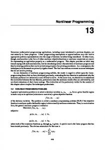
Consider the following linear program: max f (x, y) = x + y subject to 3x + 2y ≤ 6 1 x+y ≤2 2 For the present example the optimal solution is, by inspection of the LP graphical solution Fig. 2.2, the point � ∗ � ! 1 " x1 3 x∗ = = (2.165) x∗2 2 One can easily verify the Kuhn-Tucker conditions hold at this point. To do so, it is helpful to restate the problem as follows: min f (x, y) = −x − y
(2.166)
g1 (x, y) = 3x + 2y − 6 ≤ 0
(2.167)
1 x+y−2≤0 2
(2.168)
subject to
g2 (x, y) =
60
2. Elements of Nonlinear Programming
Figure 2.2: LP Graphical Solution
We note that � ∇f (x, y)
=
∇g1 (x, y)
=
�
−1 −1 3 2
� (2.169)
� (2.170)
⎛
⎞ 1 = ⎝ 2 ⎠ 1
∇g2 (x, y)
(2.171)
The Kuhn-Tucker identity is � ∇f (x1 , x2 ) + λ1 ∇g1 (x1 , x2 ) + λ2 ∇g2 (x1 , x2 ) = That is, �
−1 −1
�
� + λ1
3 2
�
0 0
� (2.172)
⎛
⎞ 1 � � 0 + λ2 ⎝ 2 ⎠ = 0 1
(2.173)
61
2.9. Numerical and Graphical Examples
The complementary slackness conditions are λ1 g1 (x1 , x2 ) =
0 λ1 ≥ 0
(2.174)
λ2 g2 (x1 , x2 ) =
0 λ2 ≥ 0
(2.175)
Note that the binding constraints define the set # � � $ 3 I = i : gi 1, = 0 = {1, 2} 2
(2.176)
and we must find multipliers that obey λ1 , λ2 ≥ 0
(2.177)
It is easy to solve the above system and show λ1 =
1 1 > 0, λ2 = > 0 4 2
(2.178)
Hence x∗ satisfies the Kuhn-Tucker conditions. Because the problem is a linear program, it is a convex program. Therefore, the Kuhn-Tucker conditions are not only necessary but also sufficient, making x∗ a global solution.
2.9.2
NLP Graphical Example
Consider the following nonlinear program min f (x1 , x2 ) = (x1 − 5)2 + (x2 − 6)2
(2.179)
subject to g1 (x1 , x2 ) =
1 x1 + x2 − 3 ≤ 0 2
g2 (x1 , x2 ) = x1 − 2 ≤ 0
(2.180) (2.181)
The graphical solution presented in Fig. 2.3, following the procedure described above, identifies (2, 2) as the globally optimal solution with a corresponding objective function value of 25. Note that � � −8 ∇f (2, 2) = (2.182) −6 ⎛ ⎞ 1 ∇g1 (2, 2) = ⎝ 2 ⎠ (2.183) 1 ∇g2 (2, 2) =
� � 1 0
(2.184)
2. Elements of Nonlinear Programming
62
Figure 2.3: NLP Graphical Solution
The Kuhn-Tucker identity is �
−8 −6
�
⎛
⎞ 1 � � � � 0 1 ⎝ ⎠ 2 + λ1 = + λ2 0 0 1
(2.185)
The complementary slackness conditions are λ1 g1 (x1 , x2 ) =
0 λ1 ≥ 0
(2.186)
λ2 g2 (x1 , x2 ) =
0 λ2 ≥ 0
(2.187)
and I = {i : gi (1, 2) = 0} = {1, 2} =⇒ λ1 , λ2 ≥ 0
(2.188)
Solving the above linear system (2.185) yields multipliers of the correct sign: λ1
= 6>0
(2.189)
λ2
= 5>0
(2.190)
63
2.9. Numerical and Graphical Examples
Consequently, the Kuhn-Tucker conditions are satisfied. Because the program is convex with a strictly convex objective function, we know that the KuhnTucker conditions are both necessary and sufficient for an unique global optimum. So, even without further analysis, we know (2, 2) is the unique global optimum.
2.9.3
Nonconvex, Nongraphical Example
Consider the nonlinear program min f (x1 , x2 ) = −x1 + 0x2
(2.191)
g1 (x1 , x2 ) = (x1 )2 + (x2 )2 − 2 ≤ 0
(2.192)
g2 (x1 , x2 ) = x1 − (x2 )2 ≤ 0
(2.193)
subject to
Note that the feasible region of this mathematical program is not convex; hence, we will have to enumerate all the combinations of binding and nonbinding constraints in order to solve it using the Kuhn-Tucker conditions alone. We begin by observing that � � −1 (2.194) ∇f (x1 , x2 ) = 0 � ∇g1 (x1 , x2 ) = � ∇g2 (x1 , x2 ) =
2x1 2x2
�
1 −2x2
(2.195) �
The Kuhn-Tucker identity is � � � � � � � � −1 2x1 1 0 + λ1 + λ2 = 0 2x2 −2x2 0
(2.196)
(2.197)
from which we obtain the equations kti1 : −1 + 2λ1 x1 + λ2 = 0
(2.198)
kti2 : (λ1 − λ2 ) x2 = 0
(2.199)
The complementary slackness conditions are csc1
: λ1 g1 (x1 , x2 ) = 0 λ1 ≥ 0
(2.200)
csc2
: λ2 g2 (x1 , x2 ) = 0 λ2 ≥ 0
(2.201)
2. Elements of Nonlinear Programming Symbol/Operator ⊕ =⇒ � dno
64
Meaning consider two statements the implication of such a consideration a contradiction has occurred does not occur
Table 2.1: Some Symbols and Operators
Because there are N = 2 inequality constraints, there are 2N = 22 = 4 possible cases of binding and nonbinding constraints: ⎫ ⎪ Case g1 g2 ⎪ ⎪ ⎪ I 0] =⇒ csc1 and csc2 satisfied =⇒ % & T T xB = (1, 1) , xC = (1, −1) are valid Kuhn-Tucker points .
65
2.9. Numerical and Graphical Examples
The global optimum is found by noting � � f� xA� = 0 � B� � � f x = f xC = −1 < f xA
(2.203)
which means xB , xC are alternative global minimizers. Note also that xA is not a local minimizer.
2.9.4
A Convex, Nongraphical Example
Let us now consider the mathematical program min f (x1 , x2 ) = 0x1 − x2
(2.204)
g1 (x1 , x2 ) = (x1 )2 + (x2 )2 − 2 ≤ 0
(2.205)
g2 (x1 , x2 ) = −x1 + x2 ≤ 0
(2.206)
subject to
Note that this problem is a convex mathematical program since the objective function is linear and the inequality constraint functions are convex. We know the Kuhn-Tucker conditions will be both necessary and sufficient for a nonunique global minimum. This means that we need only find one case of binding and nonbinding constraints that leads to non-negative inequality constraint multipliers in order to solve (2.204)–(2.206) to global optimality. We begin by observing that � � 0 (2.207) ∇f (x1 , x2 ) = −1 � ∇g1 (x1 , x2 )
=
∇g2 (x1 , x2 )
=
�
2x1 2x2 −1 1
� (2.208) �
The Kuhn-Tucker identity is � � � � � � � � 0 0 2x1 −1 + λ1 = + λ2 2x2 −1 0 1
(2.209)
(2.210)
from which we obtain the equations kti1 : 2λ1 x1 − λ2 = 0
(2.211)
kti2 : −1 + 2λ1 x2 + λ2 = 0
(2.212)
2. Elements of Nonlinear Programming
66
The complementary slackness conditions are csc1
: λ1 g1 (x1 , x2 ) = 0 λ1 ≥ 0
(2.213)
csc2
: λ2 g2 (x1 , x2 ) = 0 λ2 ≥ 0
(2.214)
Since the present mathematical program has two constraints, the table (2.202) still applies. Let us posit that both constraints are binding, so that the following analysis applies: & % Case IV: g1 = (x1 )2 + (x2 )2 − 2 = 0 ⊕ [g2 = −x1 + x2 = 0] =⇒ [x∗1 = x∗2 = 1] ⊕ [kti1, kti2] =⇒[2λ1 − λ2 = 0, −1 + 2λ1 + λ2 = 0] =⇒ ( ' 1 1 λ1 = > 0, λ2 = > 0 =⇒ [csc1 and csc2 are satisfied] =⇒ 4 2 % & T T x∗ = (x∗1 , x∗2 ) = (1, 1) is a global minimizer However, since the objective function is only convex and not strictly convex, we cannot ascertain without analyzing the three remaining cases whether this global minimizer is unique. The reader may verify that the other three cases T lead to contradictions, and thereby determine that x∗ = (1, 1) is a unique global solution.
2.10
One-Dimensional Optimization
The simplest optimization problems involve a scalar function of one variable, θ : �1 −→ �1 . As is well known, in some cases we can solve such problems by finding the zero of the derivative. Unfortunately, in practice, often one cannot find the zero analytically and must, instead, resort to numerical methods. The algorithms for solving these problems are commonly referred to as line search methods. Our specific concern is with problems of the form: min θ(x)
2.10.1
subject to
L≤x≤U
(2.215)
Derivative-Free Methods
These methods iteratively reduce an interval of uncertainty, [a, b], that is initially equal to [U, L]. They terminate when the interval of uncertainty reaches a desired length. Since it is sometimes difficult to either know or calculate the derivative of θ, these methods reduce the level of uncertainty at iteration k by evaluating θ at two points in the interval, λk and μk . The viability of this approach can be summarized as follows:
67
2.10. One-Dimensional Optimization
Theorem 2.23 Let θ : � −→ � be strictly quasiconvex over [a, b]. Let λ, μ ∈ [a, b] with λ < μ. (i) If θ(λ) > θ(μ) then θ(z) ≥ θ(μ) for all z ∈ [a, λ). (ii) If θ(λ) ≤ θ(μ) then θ(z) ≥ θ(λ) for all z ∈ (μ, b]. Proof. (i) Suppose θ(λ) > θ(μ) and z ∈ [a, λ) and assume that θ(z) < θ(μ). It follows from the strict quasiconvexity of θ that θ(λ) < max{θ(z), θ(μ)} since λ is a convex combination of z and μ. Now, by assumption, max{θ(z), θ(μ)} = θ(μ). So, θ(λ) < θ(μ) which is a contradiction. (ii) This portion of the result can be demonstrated in a similar fashion. Using Theorem 2.23, one can create a variety of different methods by varying the way in which λ and μ are selected. The golden section method generates one new test point for each iteration and identifies another test point by either setting λk+1 = μk or μk+1 = λk . That is: Case 1: θ(λk ) > θ(μk ) ak+1 = λk λk+1 = μk μk+1 is in [μk , bk ) bk+1 = bk Case 2: θ(λk ) ≤ θ(μk ) ak+1 = ak λk+1 is in (ak , λk ] μk+1 = λk bk+1 = μk The golden section method chooses the new test point in a way that ensures the length of the new interval of uncertainty does not depend on the outcome of the test at the current iteration. That is, it chooses the test point to ensure that: bk − λk = μk − ak . (2.216) It accomplishes this by choosing λk and μk as follows: λk = ak + (1 − α)(bk − ak )
(2.217)
μk = ak + α(bk − ak )
(2.218)
2. Elements of Nonlinear Programming
68
for α = 0.618 which is the golden ratio minus 1. (The golden ratio, sometimes known as the divine proportion, has connections with many aspects of mathematics √ and can be motivated in a variety of different ways. It is the value 1 (1 + 5).) Since, at each iteration, the interval of uncertainty is reduced by 2 a factor of 0.618, it follows that: (bk − ak ) = (b1 − a1 ) · 0.618k−1
(2.219)
The Fibonacci method also generates one new test point each iteration, but it allows the reduction in the interval of uncertainty to be different for each iteration. In particular, letting Fk denote the kth Fibonacci number (where F0 = 0, F1 = 1, and Fk = Fk−1 + Fk−2 ), it uses the following rules: Case 1: θ(λk ) > θ(μk ) ak+1 = λk λk+1 = μk μk+1 = ak+1 + (Fn−k−1 /Fn−k )(bk+1 − ak+1 ) bk+1 = bk Case 2: θ(λk ) ≤ θ(μk ) ak+1 = ak λk+1 = ak+1 + (Fn−k−2 /Fn−k )(bk+1 − ak+1 ) μk+1 = λk bk+1 = μk Since, at each iteration, the interval of uncertainty is reduced by a factor of Fn−k /Fn−k+1 , it follows that: (bk − ak ) = (b1 − a1 )/Fn .
2.10.2
(2.220)
Bolzano Search
If θ is differentiable and quasi-convex on [L, U ] then we can use the derivative of θ at a test point to reduce the interval of uncertainty. Letting xk denote that (single) test point at iteration k, one can proceed as follows: Case 1: dθ/dxk < 0 ak+1 = xk xk+1 is in [xk , bk )
69
2.10. One-Dimensional Optimization bk+1 = bk Case 2: dθ/dxk > 0 ak+1 = ak xk+1 is in (an , xk ] bk+1 = xk
The algorithm presented above enjoys the following convergence result: Theorem 2.24 Let {(ak , bk )} denote the sequence generated by Bolzano search, with bk ≥ ak . Then, we have (a)
(bk − ak ) = (b1 − a1 )/2k
(b) When k becomes sufficiently large, the sequence {ak − bk } converges to zero. Proof. We separately consider the two cases identified in the theorem. To show (a), it suffices to show, in both cases, we have bk+1 − ak+1 =
b k − ak 2
Evidently, for Case 1 we have ak+1 =
ak + b k 2
bk+1 = bk Thus, bk+1 − ak+1 =
bk −ak . 2
(2.221) (2.222)
Similarly, for Case 2 we have bk+1 =
ak + b k 2
ak+1 = ak
(2.223) (2.224)
k . Part (b) is an immediate result of Part (a). Thus, bk+1 − ak+1 = bk −a 2 The proof is complete.
2.10.3
Newton’s Method
Newton’s method was originally developed for finding the roots of a function. However it is clear that it can also be used to solve one-dimensional optimization problems simply by finding the first real root of the derivative of the
70
2. Elements of Nonlinear Programming
objective function. There are many ways to motivate Newton’s method. We will start by considering the following second-order approximation of θ at λk : 1 q(λ) = θ(λk ) + θ� (λk )(λ − λk ) + θ�� (λk )(λ − λk )2 2
(2.225)
Our goal at iteration k is to choose λk+1 in such a way that q � (λ) = 0. Since: q � (λ) = θ� (λk ) + θ�� (λk )(λ − λk ) we have: λk+1 = λk −
2.10.4
(2.226)
θ� (λk ) θ�� (λk )
(2.227)
Discretized Newton Methods
Based on (2.227), we may view Newton’s method as taking steps along the real line by writing it as follows: λk+1 = λk − θ�� (λk )−1 θ� (λk )
(2.228)
One can discretize this process as follows: '
λk+1
θ� (λk + hk ) − θ� (λk ) = λk − hk
(−1
θ� (λk )
(2.229)
In the regula falsi method, hk = λ − λk for some fixed λ, which leads to: '
λk+1
θ� (λ) − θ� (λk ) = λk − (λ − λk )
(−1
θ� (λk )
(2.230)
In the secant method, hk = λk−1 − λk , which leads to: '
λk+1
2.11
θ� (λk−1 ) − θ� (λk ) = λk − (λk−1 − λk )
(−1
θ� (λk )
(2.231)
Descent Algorithms in �n
For a convex mathematical program with a differentiable objective function and differentiable constraints, a particularly effective solution method is based on the notion of a feasible direction of descent introduced via Definitions 2.4–2.6. The algorithm may be stated as follows: Generic Feasible Direction Algorithm Step 0. (Initialization) Determine x0 ∈ X. Set k = 0.
2.11. Descent Algorithms in �n
71
Step 1. (Feasible direction of descent determination) Determine a feasible direction of descent. Find dk such that xk + θdk ∇[Z(xk )]T dk
∈
X ∀θ ∈ [0, 1]
< 0
Step 2. (Step size determination) Step size determination. Find the optimal step size θk where θk = arg min{Z(xk + θdk ) : 0 ≤ θ ≤ 1} Set xk+1 = xk + θk dk . Step 3. (Stopping test) For ε ∈ �1++ , a preset tolerance, if max |xk+1 − xkij | < ε ij
(i,j)∈A
stop; otherwise set k = k + 1 and go to Step 1. We will again encounter the above algorithm in Chap. 4. For now it is only necessary to note the algorithm’s simplicity and comment that one of its most commonly encountered varieties determines the feasible direction of descent using the notion of a minimum norm projection. The minimum norm projection of a vector v onto the set X is denoted as PX (v) and defined by # $ subject to x ∈ X (2.232) PX (v) = arg min �v − x� where �.� denotes the chosen norm. It is also important to recognize that the solution of 1 1 2 T min (v − x) ≡ (v − x) (v − x) 2 2 subject to x∈X is equivalent to (2.232). Of special importance to our discussion of algorithms in subsequent chapters is the minimum norm projection for the special case when X = {x ∈ �n : L ≤ x ≤ U }
(2.233)
where L, U ∈ �n++ are exogenous constant vectors representing lower and upper bounds. The associated minimum norm projection is a solution of this mathematical program: 1 2 min (v − x) 2
72
2. Elements of Nonlinear Programming subject to x−U
≤
0
(α)
L−x ≤
0
(β)
The problem’s Kuhn-Tucker conditions are x−v+α−β
=
0
αT (x − U ) =
0
β T (L − x)
=
0
α ≥
0
≥
0
β
We may relax the original constraints and employ the Kuhn-Tucker conditions to state the solution of problem’s optimality conditions as ⎧ ' (U ⎨ v if L < x < U L if x≤L x= ≡ v ⎩ L U if x≥U where, on the right side of the above expression, x is now viewed as the unconstrained solution of the program. If there are only nonnegativity constraints, the program of interest is min
1 2 (v − x) 2
subject to −x ≤ 0 Its solution may be conveniently summarized as # ' ( v if x > 0 x= = max (0, v) ≡ v 0 x≤0 + where x is again the unconstrained solution.
2.12
References and Additional Reading
Armacost, R., & Fiacco, A. V. (1974). Computational experience in sensitivity analysis for nonlinear programming. Mathematical Programming, 6, 301–326. Armacost, R., & Fiacco, A. V. (1978). Sensitivity analysis for parametric nonlinear programming using penalty methods. Computational and Mathematical Programming, 502, 261–269.
73
2.12. References and Additional Reading
Avriel, M. (1976). Nonlinear programming: Analysis and applications. Englewood Cliffs, NJ: PrenticeHall. Bazarra, M. S., Sherali, H. D., & Shetty, C. M. (2006). Nonlinear programming: Theory and algorithms. Hoboken, NJ: John Wiley Fiacco, A. V. (1983) Introduction to sensitivity and stability analysis in nonlinear programming, (367 pp.) New York: Academic. Fiacco, A. V. (1973). Sensitivity analysis for nonlinear programming using penalty methods. Technical Report, Serial no. T-275, Institution for Management Science and Engineering, The George Washington University. Fiacco, A. V., & McCormick G. P. (1968). Nonlinear programming: Sequential unconstrained minimization techniques. New York: John Wiley. Hestenes, M. R. (1975). Optimization theory: the finite dimensional case. (464 pp.) New York: Wiley. Mangasarian, O. (1969). Nonlinear programming. New York: McGraw-Hill.