Bowen Hua, Student Member, IEEE, Zhaohong Bie, Senior Member, IEEE, Cong Liu, ... C. Liu is with Argonne National Laboratory, Lemont, IL 60439 USA.
3490
IEEE TRANSACTIONS ON POWER SYSTEMS, VOL. 28, NO. 3, AUGUST 2013
Eliminating Redundant Line Flow Constraints in Composite System Reliability Evaluation Bowen Hua, Student Member, IEEE, Zhaohong Bie, Senior Member, IEEE, Cong Liu, Member, IEEE, Gengfeng Li, and Xifan Wang, Fellow, IEEE
Abstract—Reliability evaluation of composite systems involves extensive calculations. Current solutions to this computational burden have mainly focused on extracting failure states from the state space. Instead, the evaluation of failure states is accelerated by methods presented in this paper. The scale of optimizations required for generation redispatching and/or load shedding in failure states is reduced by eliminating redundant line flow constraints. First, a sufficient and necessary condition for a line flow constraint to be redundant is established in the form of a linear programming problem, based on the concept of steady-state security region (SSR). Then, two redundancy elimination methods are proposed—a conservative one based on a heuristic, and a radical one based on an analytical condition. Numerical tests are conducted on IEEE-RTS79 and a real-life system. More than half of the line flow constraints are eliminated by the conservative method and nearly 90% by the radical method. The proposed methods can be used in conjunction with most of the existing acceleration techniques to further improve efficiency. Index Terms—Composite system reliability, linear programming, optimal power flow, redundant constraints.
I. INTRODUCTION
P
ROBABILISTIC methods have been successfully applied to composite generation and transmission system reliability evaluation [1], [2]. Two main probabilistic approaches, the state enumeration method (SEM) and Monte Carlo simulation (MCS), are extensively used. Each of them involves three steps: state sampling, state evaluation, and indices updating. In SEM, states are selected based on a pre-defined contingency list [3]. The MCS approach differs from SEM by selecting system states using the concept of probability of occurrence. Both success and failure states are sampled in MCS. The main advantages of this method include its robustness to the dimension of the problem, capability to handle contingencies of all orders,
Manuscript received October 20, 2012; revised January 13, 2013; accepted February 15, 2013. Date of publication March 18, 2013; date of current version July 18, 2013. This work was supported by the National High Technology Research and Development Program of China (863 Program) under Grant 2012AA050201. Paper no. TPWRS-01174-2012. B. Hua, Z. Bie, G. Li, and X. Wang are with the State Key Laboratory of Electrical Insulation and Power Equipment, Department of Electrical Engineering, Xi’an Jiaotong University, Xi’an, Shaanxi, 710049, China (e-mail: zhbie@mail. xjtu.edu.cn). C. Liu is with Argonne National Laboratory, Lemont, IL 60439 USA. Color versions of one or more of the figures in this paper are available online at http://ieeexplore.ieee.org. Digital Object Identifier 10.1109/TPWRS.2013.2248762
and simplicity in accommodating various power system models and operation modes. However, it has a limitation: it requires that a large number of system states be sampled before the indices converge. This issue was further exacerbated by increasingly interconnected power systems with relatively high reliability. The improvement of the computational efficiency of composite system reliability evaluation with MCS is attracting widespread interest. Some of the efforts include the following: • Variance reduction techniques such as stratified sampling, importance sampling, and fission roulette method [4]–[6]. • State-space pruning [7], [8]. • State-space partitioning method [9]. • Intelligent operating state classification method based on artificial neural networks (ANN) and least squares support vector machine (LSSVM) [10]–[12]. • population-based intelligent search (PIS) methods using genetic algorithms (GAs), particle swarm optimization (PSO), and artificial immune system (AIS) [13]–[15]. • Parallel and distributed computing [16]. Previous research efforts have focused on extracting failure states from the system state space because most states sampled in a standard MCS are successes. Variance reduction techniques alter the sampling process to obtain more failure states. State space pruning and partitioning methods modify the state space in order to obtain a higher density of failure states. Instead of dealing with sampling, intelligent state classification techniques quickly identify a sampled state as a success or a failure, so that only failures are thoroughly examined. Population-based methods directly search the state space for states that contribute most to the indices, rather than sampling the state space. Existing speedup techniques have centered on the first step of the reliability evaluation, state sampling. In the second step, state evaluation, an optimal power flow (OPF) is usually conducted to determine post-contingency remedial actions of a deficit state. An AC load flow model turns the OPF into a nonlinear programming, which is usually non-convex and NP-hard [17]. Moreover, the robustness of many AC OPF algorithms is not satisfactory when multiple outages happen. Divergence could take place in severely deficit states [1]. Therefore, a DC load flow model is commonly used, which makes this OPF a linear programming (LP) problem. Inevitably, a full state evaluation with an OPF is performed for a failure state. To date, accelerating the evaluation of failure states is a problem that has not been addressed. Zhai et al. [18] presented an inspiring method for fast identification of inactive security constraints. However, it is conducted in the context of
0885-8950/$31.00 © 2013 IEEE
3491
HUA et al.: ELIMINATING REDUNDANT LINE FLOW CONSTRAINTS IN COMPOSITE SYSTEM RELIABILITY EVALUATION
unit commitment problems. This paper sheds new light on simplification of the OPFs conducted for the failure states by eliminating redundant line flow constraints. As a matter of fact, many line flow constraints are redundant in the operation of a composite system. If these constraints could be eliminated, the scale of the OPF problem is reduced, which facilitates the evaluation of failure states. In an attempt to define a redundant line flow constraint, the concept of steady-state security region (SSR) [19] is introduced. Our paper defines SSR as all feasible combinations of power injections and load demands for which power flow equations and security constraints are satisfied. On the basis of this definition, a line flow constraint is defined as redundant if it can be eliminated without changing the SSR. Such a redundant constraint is inactive for all feasible generation and load statuses. Thus, elimination of redundant constraints will not change the solution to the OPF problem. A sufficient and necessary condition is established for ensuring that a line flow constraint is redundant based on a DC load flow model. Then, a heuristic that identifies a large part of the redundant line flow constraints is developed. However, this heuristic is relatively conservative. A radical method is proposed based on an analytical condition, yet at the expense of OPF re-calculation. In our case studies, a non-sequential (state-sampling) MCS is conducted on original and modified IEEE-RTS79, as well as a real-life system in Northwestern China. We must note that the proposed methods are also applicable to sequential MCS, pseudo-simulations and SEM. At the same time, they are compatible with any one of the techniques mentioned at the beginning of this section to further improve the efficiency of composite system reliability evaluation. The remainder of this paper is organized as follows. Section II provides the problem formulation. Redundant constraint elimination methods are presented in the third section. Numerical testing results are analyzed in Section IV and conclusions follow.
vector of bus load demands (positive); vector of maximum bus load demands; load demand at bus ; vector of real power injections of generators; vector of maximum real power injections; power injection at bus ; PTDF
power transfer distribution factor matrix; vector of maximum line flow levels; vector of minimum line flow levels (negative).
(1) At first sight, this formulation might seem different from the more common form as seen in [1] and [8]. However, they are essentially the same. DC load flow equations are implicitly expressed in PTDF matrix and the power balance equation. The load levels at each bus are variable, implying possible load shedding. B. Definition of a Redundant Line Flow Constraint The line flow constraints and the power balance equation determine feasible combinations of power injections and load demands of the system (i.e., the SSR). To generalize the question, remove the objective function in OPF problem (1) and consider the following system:
II. PROBLEM FORMULATION An OPF formulation minimizing load curtailment is described in this section. The definition of a redundant constraint is then given.
(2)
A. Generation Redispatching and/or Load Shedding The optimization for generation redispatching and/or load shedding, which is conducted in the state evaluation process, is formulated as a DC OPF with an objective function of minimizing load curtailment. The system is at its initial state where no outage has yet occurred. To aid analysis, generation-shift sensitivity factors, or power transfer distribution factors (PTDFs) are introduced. Detailed calculation of these factors can be found in [20]. Some notations are introduced as follows, and the DC OPF problem is formulated as shown in (1): number of buses in the system; bus index,
;
number of transmission lines;
The two line flow constraint vectors are the focus of attention here. Therefore, the system described in (2) is denoted by . In addition, the following notations are introduced: set of all feasible combinations of system ; th element of ;
and
for
vector obtained by removing ; th row of PTDF, an vector of sensitivity factors for transmission line ; matrix obtained by eliminating from PTDF.
3492
IEEE TRANSACTIONS ON POWER SYSTEMS, VOL. 28, NO. 3, AUGUST 2013
Definition: A line flow constraint described in the following (3) is defined as redundant to system condition expressed in (4) is satisfied:
if and only if the (4)
Equation (4) implies that the following conditions must hold: (5) (6) Equation (5) is naturally satisfied because the removal of one line flow constraint can only expand the SSR. Equation (6) is thus the center of focus. By this definition, a line flow constraint is redundant if and only if the SSR of the system remains unchanged after this constraint is eliminated. Also, this redundancy is not defined for a specific solution or a specific objective function, but for all feasible generation and load status. For a minimum line flow constraint, the definition is exactly the same.
which is the same as the eliminated constraint. This indicates that any feasible solution to system is also feasible to system . Equation (6) therefore is satisfied. According to the definition in Section II, constraint (3) is redundant to system . Necessity: If the constraint is redundant, (6) is satisfied. Any solution within is a solution to . Because constraint (3) should be met for any solution in , the maximum value of the objective function, which is the same as the left side of constraint (3), should be less than . Therefore, holds. Note that a maximum line flow constraint is chosen as the example again. For a minimum line flow constraint, the LP problem tries to minimize the objective function, rather than maximizing it. The established condition should be changed into . Theorem 1 is theoretically sufficient and necessary. However, it is of little practical use because of the formidable amounts of time consumed by a series of LPs. Theorem 2: Consider the LP following problem:
III. ELIMINATING REDUNDANT CONSTRAINTS If most of the line flow constraints are redundant and identified efficiently, the calculation of OPF problem (1) as well as the whole reliability evaluation will be considerably facilitated. Two elimination methods are developed in this section. Then, the method to integrate constraint elimination into reliability evaluation procedure is given. A. Conservative Elimination Initially, a sufficient and necessary condition for a line flow constraint to be redundant is established, as well as a simpler sufficient condition. More importantly, a heuristic based on the sufficient condition is developed, by which a large part of the redundant constraints can be identified quickly. Theorem 1: Consider the following LP problem:
(9) A line flow constraint expressed in (3) is redundant to system if . Proof: All line flow constraints are taken away in (9). Therefore, the feasible region for problem (9) is a superset of that for problem (7). Thus, it is clear that , which implies that . Based on Theorem 1, this line flow constraint is redundant to . Theorem 2 provides a sufficient condition for a redundant constraint. The objective function could be interpreted as the maximum possible power flow over certain transmission line with all line flow constraints neglected. If maximum possible line flow is still less than the limit, this line flow constraint is undoubtedly redundant. However, Theorem 2 is still an LP problem, only with fewer constraints. It would be desirable to discover a method that identifies redundant constraints without solving any optimization problem. In an effort to obtain such a method, is sorted in descending order. Let be a permutation of such that
(7)
(10)
The constraint expressed in (3) is redundant to system if and only if . Proof. Sufficiency: All feasible solutions to the system defined in (7) constitute . If , then for any solution within , the following equation holds:
is satisfied. Consider the heuristic shown in Fig. 1. Given that the PTDF matrix is already obtained, this heuristic runs in time for a single constraint. In the end, is inevitably reached. Assume that , and the following results are obtained:
(8)
(11)
HUA et al.: ELIMINATING REDUNDANT LINE FLOW CONSTRAINTS IN COMPOSITE SYSTEM RELIABILITY EVALUATION
3493
Theorem 3: Assume that is determined by the above method. If the following condition is satisfied:
(17) the line flow constraint expressed in (3) is redundant to system . Proof: We will first prove that and obtained by (11)–(16) is an optimal solution to LP (9). Consider the dual program of (9):
.. .
Fig. 1. Heuristic for determining .
(12)
.. .
(13) (14)
.. .
(15) .. . (16) By substituting above equations into the objective function of (9), we can get an analytical expression, which will be later proved to be the optimal value of the objective function. Here we provide a physical interpretation for this heuristic. Initially, all power injections and load demands are set at zero. Available generation and load for all nodes are set at their maximum . Two pointers, and are defined, with at the beginning of the sorted vector and at the bottom, maximizing , and thereby maximizing the increase of line flow. Maximum line flow is reached by gradually injecting generation and load. Notice that power balance should always be met between generation and load. Keep injecting as much power at as possible, and add the same amount of load demand at . If available generation at a certain bus is zero, moves rightward along the permutation . Otherwise, moves leftward. This process goes on until the marginal increase of line flow caused by any amount of power injection and matched load demand is zero . A mathematically rigorous justification is shown below.
(18) A feasible solution to the dual problem is shown in the following:
(19) Equations (11)–(16) also construct a feasible solution to the primal program (9). These two solutions satisfy the conditions of the complementary slackness theory [21], which indicates that the two solutions are both optimal solutions of the primal and dual program.
3494
IEEE TRANSACTIONS ON POWER SYSTEMS, VOL. 28, NO. 3, AUGUST 2013
Bus 1. Power injection at Bus 4 and load at Bus 1 are set at 1.6. Then, moves to Bus 3. The generation at Bus 4 is increased to 5, and the load at Bus 3 is set at 3.4. Now the line flow reaches its maximum, and . Further calculation would reveal that the other 9 line flow constraints are all redundant. Notice that is not necessarily equal to , because Theorem 3 is based on Theorem 2, which is a sufficient condition. In a more complicated power system, is probably lower than .
Fig. 2. Five-bus system.
B. Radical Elimination
TABLE I BRANCH PARAMETERS FOR THE 5-BUS SYSTEM
According to the duality theory [21], the objective function of the primal and dual program is equal in this scenario. Substitute both of the two optimal solutions into their objective functions respectively and we have
The elimination method described in Theorem 3 is relatively conservative, although theoretically sufficient. Some of the redundant line flow constraints are not identified. Notice that all load demands are variable in the OPF problem (1). Intuitively, a lower load level usually leads to a less stressed transmission network. Suppose that one line flow constraint is redundant to the system at peak load level: it would probably still be redundant after a certain amount of load shedding. Therefore, it would be reasonable to develop an elimination approach based on fixed peak load level. It is hoped that the number of constraints eliminated will be increased. The fixed load demand at bus is designated as . The following system is given:
(20) which is exactly the same as the left side of (17). According to Theorem 2, the redundancy is validated. To deal with a minimum flow constraint, the only modification is to sort in ascending order when determining the permutation shown in (10). To better illustrate the proposed theorems and methods, here we present a 5-bus system cited from [22], as shown in Fig. 2. This is a simple system with 2 generators, 2 transformers, and 3 transmission lines. All parameters are given in per-unit. The indexing, positive directions, and line flow limits of branches are shown in Table I. In order to identify redundant line flow constraints in this system, the PTDF matrix of this system is obtained and shown below, with Bus 5 assigned as the slack bus. The indexing of the rows of this matrix is in alignment with the indexing of branches, and the indexing of rows accords with that of buses:
(21)
Consider the line flow through the positive direction of Branch 1, from Bus 2 to Bus 1. Solve LP problem (7) and we can get , which is larger than the flow limit. Thus this line flow constraint is not redundant. Same result could be achieved by Theorem 3. According to the algorithm of the heuristic, first, points at Bus 4 and at
(22)
We have the following three theorems, which are the counterparts of Theorems 1, 2, and 3, respectively. Theorem 4: Consider the following LP problem:
(23) The constraint expressed in (3) is redundant to system if and only if . Theorem 5: Consider the LP following problem:
(24) A line flow constraint expressed in (3) is redundant to system if .
HUA et al.: ELIMINATING REDUNDANT LINE FLOW CONSTRAINTS IN COMPOSITE SYSTEM RELIABILITY EVALUATION
3495
C is not theoretically rigorous. It is hoped that the reduced OPF time due to additional elimination (Area ) would outweigh the extra computational burden of possible OPF re-calculation.
D. Integration into Reliability Evaluation
Fig. 3. Redundant line flow constraints identified by different theorems.
Theorem 6: If
(25)
(26) hold for some , then a line constraint shown in (3) is redundant to system . An advantage of the radical elimination is that is determined solely by (25) rather than the previous heuristic method. Thus, the elimination procedure is simplified. However, all of the above theorems are based on system , whose load demand is assumed to be fixed. Redundancy of part of the constraints eliminated by the radical method is not theoretically rigorous. Those constraints, although eliminated, might still be violated when load demand is changed (e.g., after certain amount of load shedding). In order to reach accurate results, if there is load shedding after an OPF, those eliminated line flow constraints will be checked. If there is any violation, a re-calculation of OPF is required. Because system is simplified from , the proofs of the above three theorems are similar to their counterparts in Section III-A and thus omitted here. C. Different Sets of Redundant Line Flow Constraints Fig. 3 shows the overlapping sets of redundant constraints identified by different theorems. The set of all line flow constraints is divided into five parts. The most accurate way to achieve elimination is to solve (7) in Theorem 1 exhaustively, by which line flow constraints represented by Area A+B+D are eliminated. However, the amount of time consumed solving a series of LPs is formidable. If the conservative method is adopted, only constraints in Area A are eliminated. If the radical method is employed, constraints in Area are eliminated, though the redundancy of constraints in Area
The DC OPF formulation stated in Section II is based on the initial state where no outage occurs. This is unrealistic in reliability evaluation. 1) Outages in the Generation System: Consider LP problem (18). The objective function is the sum of the products of two nonnegative values ( and ), and the values of are determined by PTDF. If there is an outage of the generator at bus decreases from a positive value to zero, thereby decreasing the objective function. Thus, a line flow constraint identified as redundant to system by Theorem 3 is still redundant to the system when outages of generators occur. For the radical elimination method, the same conclusion holds. This result can be proved by investigating the dual program of (24) in a similar way. 2) Load Variation: System load level may vary in reliability assessment. For instance, a chronological load curve is used in a sequential MCS. Considering problem (18) and the dual of (24), we could easily reach the conclusion that a line flow constraint that identified as redundant to system is still redundant when load level decreases. In this paper, the highest possible load of each node is used in the constraint elimination process. 3) Outages in the Transmission System: An outage of transmission lines or transformers alters the network configuration, as well as the PTDF matrix. Nothing could be done to rectify the problem but a re-identification of redundancy. Notice that the force outage rate (FOR) of a transmission line or a transformer is relatively low. Therefore, it would be reasonable to perform constraint eliminations for the initial network configuration and all of the N-1 contingencies. (Here N-1 means first-order failure in the transmission network.) An alternative would be to conduct eliminations for part of the N-1 contingencies with contingency-ranking techniques. For a certain network configuration, the calculation of the PTDF matrix is the most time-consuming part because an X matrix, the inverse of the nodal susceptance matrix B, is needed. To tackle this challenge, a branch addition method [22] could be utilized to facilitate this process. After solving the X matrix of original network configuration, the X matrices of different transmission contingencies could be obtained by making simple modifications to the original one. 4) Modifications to the Evaluation Process: It is desirable to use line flow constraint elimination as a preprocessing method. Before reliability evaluation, the set of preprocessed transmission states should be determined, and the constraint elimination is conducted only for once. According to the conclusion in Part 1) of this section, outages in the generation system will not influence the redundancy of eliminated line flow constraints. As shown in Fig. 4, the only modification of the proposed methods to reliability evaluation is in the state evaluation procedure. Our method is therefore compatible with various reliability evaluation techniques.
3496
IEEE TRANSACTIONS ON POWER SYSTEMS, VOL. 28, NO. 3, AUGUST 2013
TABLE II TESTING RESULTS FOR IEEE-RTS79
Fig. 4. Modified state evaluation process.
IV. CASE STUDY Numerical tests are conducted on the original and modified IEEE-RTS79, as well as a real-life power system. All tests are performed on a MATLAB platform, with a PC consisting of a 1.8-GHz processor and 2 GB of RAM. Non-sequential MCS is used. In state sampling, failures of both the generation and transmission systems are considered. In state evaluation, a power flow is solved first to check whether security constraints are violated. Then, the OPF model described in Section II is solved when necessary by MIPS, a MATLAB-implemented interior point solver [23]. In indices updating, two of the most commonly used power system reliability indices, loss-of-load probability (LOLP) and expected energy not supplied (EENS), are calculated. Three case studies are performed for each system. In Case 1, standard non-sequential MCS is conducted. Case 2 includes a preprocessing of the conservative elimination method. In Case 3, the radical elimination method is employed. A. Original IEEE-RTS79 IEEE-RTS79 [24] includes 24 buses, 38 transmission lines, and 32 generators. The total generation capacity is 3405 MW. The load is assumed to be constant at its peak value of 2850 MW. For the initial network configuration, redundant line flow constraints are first identified by Theorem 1. After solving 76 LP problems, we can get that only 3 line flow constraints are not redundant. They are constraints of Branch 7–8, 14–16, and 16–17 (as indexed in the single line diagram of this system in [24]), each in one direction. In case studies, we make use of redundancy information from Theorem 3 and Theorem 6. The set of preprocessed system states is defined as the initial state and all N-1 transmission contingencies where no disconnection occurs. Table II highlights that more than 70% of the line flow constraints are eliminated by the conservative method and more than 90% by the radical
method. A striking result is that for the initial network configuration, only one line flow constraint remains (line 7–8 in one direction) after a radical elimination. The seeds for the random number generator in the three cases are set to be identical for the sake of comparison. A total number of states are sampled in each case with around power flows and 19,495 optimizations performed. Of all the states that need an OPF, 96.20% contain no outage in transmission, and 3.75% include first-order transmission contingency. This means that 99.95% of the OPFs are accelerated. The number of eliminated constraints for the initial state and the average number of eliminated constraints for all the other preprocessed states (all N-1 transmission contingencies in this case) are described in Table II. The time consumed by OPFs is reduced by 25.7% when conservative elimination is used. The ratio is 31.7% for the radical method. Although most of the line flow constraints are eliminated, speedup ratios seem slightly lower than expected. The acceleration of total evaluation time is even less remarkable. This can be accounted by the relatively small scale of IEEE-RTS79. B. Modified IEEE-RTS79 The original IEEE-RTS79 is generation-deficit. It is modified to stress the transmission system. Generation capacities and load levels at all delivery points are both increased to p.u. of the original values. All other parameters remain the same. A set of ranging from 1 to 1.3 is used to study the correlation between eliminated constraints and load level. If goes higher than 1.3, at least one line flow constraint is not satisfied—even in the initial state. Fig. 5 highlights that the number of eliminated constraints is closely related to the load level. If the conservative method is chosen, this number decreases by 30.4% if increases from 1 to 1.3. For the radical method, the drop is only 5.3%, which suggests that the performance of the radical method is less sensitive to load variation. We sampled states when is set at 1.3, and 21,498 OPFs are performed. The speedup ratio for OPFs decreases to 14.2% and 29.6% for the conservative and radical elimination methods, respectively. This result reveals a positive correlation between the number of eliminated constraints and the reduction of computational time. C. Real-Life Power System in Northwestern China The proposed methods are also applied to a real-life power system in Northwestern China, which contains 773 buses, 279 generating units, and 1036 transmission lines (2072 line flow
HUA et al.: ELIMINATING REDUNDANT LINE FLOW CONSTRAINTS IN COMPOSITE SYSTEM RELIABILITY EVALUATION
3497
TABLE III TESTING RESULTS FOR THE REAL-LIFE SYSTEM
D. On OPF Re-Calculation
Fig. 5. Number of eliminated constraints with different .
Fig. 6. Diagram for the 750-kV backbone network of the real-life system and the result of constraint elimination.
Of the two proposed elimination methods, the conservative one is based on a series of sufficient theorems. Thus, no accuracy of the obtained reliability indices is lost. For the radical method, OPF re-calculation is introduced to obviate the loss of accuracy. We found that the radical method generally performs better than the conservative elimination, because the number of OPF re-calculation is negligible. Specifically, of all the 19 495 optimizations performed on the original IEEE-RTS79 in our case study, none needed re-calculation. Also, reliability evaluation of the real-life system is repeated 10 times with the same convergence criterion (coefficient of variance %), and the number of re-calculation in each evaluation varies from 3 to 22. This can be justified in part by that the redundancy of constraints in Area C of Fig. 3 is possibly erroneous only when load shedding happens. Another reasonable explanation for this result may lie in the interior point solver. Iterates of interior point methods move along the interior of the feasible region—instead of traveling from vertex to vertex around the boundary, as that of the simplex method—toward an optimal solution. It is likely that those line flow constraints that fall in Area C of Fig. 2 are not violated. Yet we cannot rule out that this conclusion is system-specific. V. CONCLUSION
constraints). Five regional grids are interconnected with 330-kV and 750-kV transmission lines. The total generating capacity is 28.8 GW. System load is set to be constant at its peak value, 22.4 GW. For the initial network configuration, 1827 line flow constraints are redundant, according to Theorem 1. The set of preprocessed system states remains the same. In the initial state, 84.03% of the line flow constraints are eliminated by the conservative method and 91.75% by the radical method. Only six line flow constraints (six transmission lines in one direction) remain in the 750-kV backbone transmission network after a conservative elimination (Fig. 6). If the radical method is employed, the two constraints of the double-circuit transmission lines between 2–7 and 1–26 are also eliminated. This result provides useful information for transmission planning by indicating crucial transmission lines that affect reliability. A total number of states are sampled in each case with 20 560 optimizations performed. And 99.8% of the optimizations are accelerated. Table III indicates that the computational time of OPFs is reduced by 31.6% with the conservative method and by 35.7% using the radical method. This result suggests that the methods presented in this paper are more beneficial for application to larger systems.
Many of the line flow constraints in a composite power system are redundant in reliability evaluation. The computational burden could be reduced if these constraints are eliminated. This paper develops two elimination methods and their effectiveness is validated through numerical tests. First, more than half of the line flow constraints are eliminated by the conservative method. Nearly 90% of the constraints are eliminated by the radical method. A downside factor regarding our methodology is that the performance is less satisfactory for transmission-deficit systems. Second, the computational time of reliability evaluation is reduced after the redundant constraints are eliminated, especially for large-scale systems. The radical method generally provides better performance. Third, the remaining constraints indicate transmission lines that are crucial to the reliability indices, providing information of weak transmission areas. Our research has succeeded in accelerating the evaluation of failure states. Nevertheless, the proposed methods are not intended to replace any of the existing speedup techniques. In fact, future work should focus on the cooperation between redundant constraint elimination and other reliability evaluation speedup techniques to further improve efficiency.
3498
IEEE TRANSACTIONS ON POWER SYSTEMS, VOL. 28, NO. 3, AUGUST 2013
REFERENCES [1] R. N. Allan and R. Billinton, “Probabilistic assessment of power systems,” Proc. IEEE, vol. 88, no. 2, pp. 140–162, Feb. 2000. [2] R. Billinton and R. N. Allan, Reliability Evaluation of Power Systems. New York, NY, USA: Plenum, 1996. [3] A. M. Rei and M. T. Schilling, “Reliability assessment of the Brazilian power system using enumeration and Monte Carlo,” IEEE Trans. Power Syst., vol. 23, no. 3, pp. 1480–1487, Aug. 2008. [4] A. C. G. Melo, G. C. Oliveira, M. M. Fo, and M. V. F. Pereira, “A hybrid algorithm for Monte Carlo/enumeration based composite reliability evaluation,” in Proc. 1991 3rd Int. Conf. Probabilistic Methods Applied to Electric Power Systems, pp. 70–74. [5] M. V. F. Pereira, M. E. P. Maceira, G. C. Oliveira, and L. M. V. G. Pinto, “Combining analytical models and Monte-Carlo techniques in probabilistic power system analysis,” IEEE Trans. Power Syst., vol. 7, no. 2, pp. 265–272, Feb. 1992. [6] Z. Bie and X. Wang, “Studies on variance reduction technique of Monte Carlo simulation in composite system reliability evaluation,” Elect. Power Syst. Res., vol. 63, no. 1, pp. 59–64, Aug. 2002. [7] C. Singh and J. Mitra, “Composite system reliability evaluation using state space pruning,” IEEE Trans. Power Syst., vol. 12, no. 1, pp. 471–479, Feb. 1997. [8] R. C. Green, L. Wang, M. Alam, and C. Singh, “State space pruning for reliability evaluation using binary particle swarm optimization,” in Proc. 2011 IEEE/PES Power Systems Conf. Expo., pp. 1–7. [9] J. He, Y. Sun, D. S. Kirschen, C. Singh, and L. Cheng, “State-space partitioning method for composite power system reliability assessment,” IET Gener., Transm., Distrib., vol. 4, no. 7, pp. 780–792, Jul. 2010. [10] M. T. Schilling, J. C. S. Souza, A. P. A. da Silva, and M. B. D. C. Filho, “Power systems reliability evaluation using neural networks,” Eng. Intell. Syst., vol. 9, no. 4, pp. 219–226, Dec. 2001. [11] M. L. da Silva, L. C. Resende, L. A. F. Manso, and V. Miranda, “Composite reliability assessment based on Monte Carlo simulation and artificial neural networks,” IEEE Trans. Power Syst., vol. 22, no. 3, pp. 1202–1209, Aug. 2007. [12] N. M. Pindoriya, P. Jirutitijaroen, D. Srinivasan, and C. Singh, “Composite reliability evaluation using Monte Carlo simulation and least squares support vector classifier,” IEEE Trans. Power Syst., vol. 26, no. 4, pp. 2483–2490, Nov. 2011. [13] N. Samaan and C. Singh, “Assessment of the annual frequency and duration indices in composite system reliability using genetic algorithms,” in Proc. IEEE PES General Meeting, 2003, vol. 2. [14] L. Wang and C. Singh, “Population-based intelligent search in reliability evaluation of generation systems with wind power penetration,” IEEE Trans. Power Syst., vol. 23, no. 3, pp. 1336–1345, Aug. 2008. [15] V. Miranda, L. de Magalhaes Carvalho, M. A. da Rosa, A. M. L. da Silva, and C. Singh, “Improving power system reliability calculation efficiency with EPSO variants,” IEEE Trans. Power Syst., vol. 24, no. 4, pp. 1772–1779, Nov. 2008. [16] C. L. T. Borges, D. M. Falcao, J. C. O. Mello, and A. C. G. Melo, “Composite reliability evaluation by sequential Monte Carlo simulation on parallel and distributed processing environments,” IEEE Trans. Power Syst., vol. 16, no. 2, pp. 203–209, May 2001. [17] J. Lavaei and S. H. Low, “Zero duality gap in optimal power flow problem,” IEEE Trans. Power Syst., vol. 27, no. 1, pp. 92–107, Feb. 2012. [18] Q. Zhai, X. Guan, J. Cheng, and H. Wu, “Fast identification of inactive security constraints in SCUC problems,” IEEE Trans. Power Syst., vol. 25, no. 4, pp. 1946–1954, Nov. 2010. [19] F. Wu and S. Kumagai, “Steady-state security regions of power systems,” IEEE Trans. Circuits Syst., vol. 29, no. 11, pp. 703–711, Nov. 1982.
[20] B. Wollenberg and A. Wood, Power Generation, Operation and Control, 2nd ed. New York, NY, USA: Wiley, 1996. [21] D. G. Luenberger and Y. Ye, Linear and Nonlinear Programming, 3rd ed. New York, NY, USA: Springer, 2008. [22] X. Wang, Y. Song, and M. Irving, Modern Power Systems Analysis. New York, NY, USA: Springer, 2008. [23] R. D. Zimmerman, C. E. Murillo-Sánchez, and R. J. Thomas, “MATPOWER: Steady-state operations, planning and analysis tools for power systems research and education,” IEEE Trans. Power Syst., vol. 26, no. 1, pp. 12–19, Feb. 2011. [24] IEEE APM Subcommittee, “IEEE reliability test system,” IEEE Trans. Power App. Syst., vol. PAS-99, pp. 2047–2054, Nov./Dec. 1979. Bowen Hua (S’12) received the B.S. degree from the School of Electrical Engineering, Xi’an Jiaotong University, Xi’an, China, in 2012. He is currently pursuing the M.S. degree in Xi’an Jiaotong University. His major research interests include power system reliability and renewable energy integration.
Zhaohong Bie (M’98–SM’12) received the B.S. and M.S. degrees from the Electric Power Department of Shandong University, Jinan, China, in 1992 and 1994, respectively, and the Ph.D. degree from Xi’an Jiaotong University, Xi’an, China, in 1998. Currently, she is a professor in the State Key Laboratory of Electrical Insulation and Power Equipment and the School of Electrical Engineering, Xi’an Jiaotong University. Her main interests are power system planning, reliability evaluation, as well as the integration of renewable energy into power systems.
Cong Liu (S’08–M’10) received the B.S. and M.S. degrees in electrical engineering from Xi’an Jiaotong University, Xi’an, China, in 2003 and 2006, respectively, and the Ph.D. degree at the Illinois Institute of Technology, Chicago, IL, USA, in 2010. Currently, he is working as an energy systems computational engineer in the Decision and Information Sciences Division of Argonne National Laboratory, Lemont, IL, USA. His research interests include numerical computation, optimization, and control of power systems.
Gengfeng Li received the B.S. degree from the School of Electrical Engineering, Xi’an Jiaotong University, Xi’an, China. He is currently pursuing the Ph.D. degree at Xi’an Jiaotong University. His major research interests include reliability evaluation of distribution systems.
Xifan Wang (F’09) received the B.S. degree from Xi’an Jiaotong University, Xi’an, China, in 1957. He is with the School of Electrical Engineering, Xi’an Jiaotong University, where he is a professor. From September 1981 to September 1983, he worked in the School of Electrical Engineering, Cornell University, Ithaca, NY, USA, as a visiting scientist. From September 1991 to September 1993, he worked at the Kyushu Institute of Technology, Kitakyushu, Japan, as a visiting professor. His research fields include power system analysis, generation planning and transmission system planning, reliability evaluation, and electricity markets.