Identifying Redundant Linear Constraints in Systems of Linear Matrix Inequality Constraints Shafiu Jibrin (
[email protected]) Department of Mathematics and Statistics Northern Arizona University, Flagstaff Arizona 86011-5717
Daniel Stover (
[email protected]) Department of Mathematics and Statistics Northern Arizona University, Flagstaff Arizona 86011-5717
Abstract. Semidefinite programming has been an interesting and active area of research for several years. In semidefinite programming one optimizes a convex (often linear) objective function subject to a system of linear matrix inequality constraints. Despite its numerous applications, algorithms for solving semidefinite programming problems are restricted to problems of moderate size because the computation time grows faster than linear as the size increases. There are also storage requirements. So, it is of interest to consider how to identify redundant constraints from a semidefinite programming problem. However, it is known that the problem of determining whether or not a linear matrix inequality constraint is redundant or not is NP complete, in general. In this paper, we develop deterministic methods for identifying all redundant linear constraints in semidefinite programming. We use a characterization of the normal cone at a boundary point and semidefinite programming duality. Our methods extend certain redundancy techniques from linear programming to semidefinite programming. Keywords: Semidefinite programming, Linear matrix inequalities, Redundancy, Normal cone. AMS Subject Classification: 90C25, 15A45, 15A39, 15A48
2 1. Introduction Semidefinite Programming is one of the most interesting and challenging areas in operations research to emerge in the last decade. Semidefinite programming problems arise in a variety of applications e.g., in engineering, statistics and combinatorial optimization ([3], [10]. A semidefinite programming problem is an extension of a linear programming problem where the linear constraints are replaced by linear matrix inequality (LMI) constraints. Semidefinite programming also generalizes quadratically constrained quadratic programming QCQP ([24]). We consider semidefinite programming program (SDP) of the following form:
SDP : min cT x s.t.
(1.1)
A(x) º 0 bj + aTj x ≥ 0 (j = 1, 2, . . . , q)
where the variable is x ∈ IRn and A(x) := A0 +
n X
xi Ai .
i=1
The problem data are the m × m symmetric matrices Ai and the vectors aj , bj , c in IRn . The variable is the vector x ∈ IRn . The constraint A(x) º 0 is called a linear matrix inequality (LMI) and A(x) º 0 means that all the eigenvalues of A(x) are nonnegative. Nestrov and Nemirovsky in 1988 [21] showed that interior-point methods for linear programs can, in principle, be generalized to convex optimization problems such as SDP’s. Many polynomial time interior point methods have been developed for solving SDP’s including ([3], [8], [25], [23]). A lot is known on both the classes of problems that SDP formulation can handle, and the best SDP algorithms to solve each class. In addition, a great deal has been learned about the limits of the current algorithms to solving SDP’s. One limitation to current SDP algorithms is that they are restricted to problems where the number of constraints are moderate [5]. This is due to the fact that the number of computations required becomes too high for large problems. In practice, the number of iterations required to solve SDP problems grows very slowly with the size of the problem [24].
3 The most important factor in the time complexity is the cost per iteration. For example, each iteration of the primal-dual algorithm described in [24] requires O(n2 (m + q)2 ) time. Significant savings in computation time can be gained if the number of constraints can be effectively reduced before the problems are solved. Furthermore, storage requirements are at least as important as the computational time complexity [9]. The second most important issue in creating a fast implementation of an interior point method is preprocessing to reduce problem size [20]. A redundant constraint is one that can be removed without changing the feasible region defined by the original system of constraints, otherwise it is called necessary. Larger SDP problems can be solved if we can identify and eliminate the redundant constraints before the problems are solved. There is always a positive result from identifying redundancy [18]. Apart from computational and storage difficulties caused by redundancy, the knowledge that a constraint is redundant might offer additional insight into the problem model or might lead to different decisions about the problem. So, it is of interest to study how to identify redundant constraints. An interesting question that naturally arises is: Can we extend all redundancy methods from linear programming to semidefinite programming? The answer is no. It has been shown that the problem of determining whether or not an LMI constraint is redundant in semidefinite programming is NP complete [17], in general. We are concerned with identifying all redundant linear constraints from the SDP (1.1). A naive approach would be to identify all the redundant linear constraints with respect to the system of the linear constraints only. Such approach would only guarantee a partial identification of all the redundant linear constraints in SDP 1.1. We assume that there is a large number of linear constraints in the problem, that is, q is large. There is abundant literature on redundancy techniques in the case of linear programming. An excellent survey of these is given in ([11],[18]). One class of the methods is called hit-and-run. These methods are probabilistic and they work by detecting the necessary constraints. There is a small chance that a constraint declared redundant by a hit-and-run method, is actually necessary. In ([17], [16]), hit-and-run redundancy detection methods were extended from linear programming to semidefinite programming. A different and relatively more expensive class of redundancy methods in linear programming are the deterministic methods. An early paper on these methods is that of
4 Balinsky [4], published in 1961. See also ([18], [11] and [12]). Deterministic methods have the advantage that they identify both necessary and redundant linear constraints with probability 1. The study of deterministic methods for identifying redundant constraints in semidefinite programming seems to be somewhat absent from the literature. A study of presolving for SDP is given in [14]. In this paper, we develop deterministic methods for the identification of all redundant linear constraints from (1.1). We use SDP duality and a characterization of the normal cone at a boundary point. Our methods generalize some of the redundancy techniques in linear programming to semidefinite programming. This work gives practical methods for identifying all redundant linear constraints in semidefinite programming.
2. Identifying Redundant Linear Constraints In this section, we present our main result for identifying all redundant linear constraints from the system of inequalities that defines the feasible region of SDP (1.1). We consider the system:
A(x) º 0
(2.1)
bj + aTj x ≥ 0 (j = 1, 2, . . . , q)
(2.2)
Let R = {x ∈ IRn : A(x) º 0, bj + aTj x ≥ 0, j = 1, 2, . . . , q} Rk = {x ∈ IRn : A(x) º 0, bj + aTj x ≥ 0, j = 1, . . . , k − 1, k + 1, . . . , q}
(2.3) (2.4)
The kth linear constraint is said to be redundant with respect to R if R = Rk . Otherwise, it is said to be necessary. It is called weakly redundant if it is redundant and its boundary {x ∈ IRn : bk +aTk x = 0} touches the feasible region R. A linear constraint whose boundary does not touch the feasible region is called strongly redundant. A redundant linear constraint that can become necessary with the removal of some other redundant constraints is called relatively redundant, otherwise it is called absolutely redundant. The
5 LMI constraint A(x) º 0 is called redundant, necessary, weakly redundant, strongly redundant, relatively redundant or absolutely redundant with respect to R in a similar way. An excellent discussion on these concepts is given in [7]. Consider the kth linear constraint in (2.2) and the following associated semidefinite programming problem:
SDPk : min aTk x s.t. x ∈ Rk The dual of SDPk is DSDPk : max −A0 • Z − s.t. Ai • Z +
q X
bj yj
j=1,j6=k q X
(aj )i yj = (ak )i (i = 1, 2, . . . , n),
j=1,j6=k
Zº0 yj ≥ 0 (j = 1 . . . , k − 1, k + 1, . . . , q), where the variables are m×m symmetric matrix Z and yj ∈ IR (j = 1 . . . , k−1, k+1, . . . , q). X A•B = aij bij is the standard inner product on the set of real matrices. We assume that: i,j
Assumption 1: SDPk is strictly feasible. Observe that if R is strictly feasible, so is each SDPk . The following theorem gives the main foundation of our methods for identifying redundant linear constraints from the system (2.1) and (2.2). THEOREM 2.1. The linear constraint bk + akT x ≥ 0 is redundant with respect to R if and only if the infimum p∗k of the objective function values of SDPk exists that satisfies bk + p∗k ≥ 0. Proof (⇒) Suppose bk + aTk x ≥ 0 is redundant. Then Rk = R, and so for each x ∈ Rk , we have bk + aTk x ≥ 0. Hence, the set {aTk x : x ∈ Rk } is bounded from below by −bk .
6 By Assumption 1, the infimum p∗k of the objective function values of SDPk exists that satisfies p∗k ≥ −bk , that is, bk + p∗k ≥ 0. (⇐) Suppose bk + aTk x ≥ 0 is necessary. Then, there exists a point x ˜ such that x ˜ ∈ Rk but bk + aTk x ˜ < 0. If the objective values of SDPk has no infimum, then the proof is done. If the infimum pk∗ of the objective function values of SDPk exists, then p∗k ≤ aTk x ˜ and hence bk + p∗k ≤ bk + aTk x ˜ < 0. 2 It is informative to note that in the above theorem, the optimal solution of SDPk may not be attained in Rk . Consider the following example from [24]: 0 0 1 0 0 1 + x2 º0 + x1 0 1 0 0 1 0 x1 ≥ 0
(1)
Clearly, x1 ≥ 0 is implied by the linear matrix inequality constraint and thus redundant. But, SDP1 has no optimal solution (x∗1 , x∗2 ) in the feasible region with x∗1 ≥ 0. Here, the dual of SDP1 is not strictly feasible. If the dual DSDPk is strictly feasible, then SDPk attains its optimal solution in Rk [15]. We assume: Assumption 2: DSDPk is strictly feasible. We remark that if DSDPk is not strictly feasible, but it has a nonempty relative interior, then an equivalent problem that is strictly feasible can be constructed by projecting the minimal face as described in [15]. We state the following corollary to Theorem 2.1: COROLLARY 2.1. The linear constraint bk + aTk x ≥ 0 is redundant with respect to R if and only if SDPk has an optimal solution x∗k in Rk that satisfies bk + aTk x∗k ≥ 0. Proof By Assumption 2, SDPk attains its optimal solution in Rk . The rest follows from Theorem 2.1. 2
Corollary 2.1 shows that all redundant linear constraints can be found by solving SDPk for k = 1, 2, . . . , q. In the next section, we provide short-cuts less expensive than solving SDPk for identifying some of the linear constraints as redundant or not. Recall that by Assumption 1, each SDPk is strictly feasible.
7 LEMMA 2.1. ([24] A point x∗k ∈ IRn is optimal to SDPk if and only if there is Z ∗ º 0 and yj∗ ≥ 0 (j = 1, . . . , k − 1, k + 1, . . . , q) such that the following KKT conditions hold: A(x∗k ) º 0, bj + aTj x∗k ≥ 0 (j = 1, . . . , k − 1, k + 1, . . . , q) P Ai • Z ∗ + qj=1,j6=k (aj )i yj∗ = (ak )i (i = 1, 2, . . . , n)
(2.5)
A(x∗k )Z ∗ = 0, (bj + aTj x∗k )yj∗ = 0 (j = 1, . . . , k − 1, k + 1, . . . , q)
(2.7)
(2.6)
PROPOSITION 2.1. Let x∗k ∈ IRn . Let rank(A(x∗k )) = r and consider an orthogonal decomposition of A(x∗k ) A(x∗k ) = [Q1 Q2 ]diag(0, . . . , 0, λ1 , λ2 , . . . , λr )[Q1 Q2 ]T . where λ1 , . . . , λr are the nonzero eigenvalues of A(x∗k ). Then x∗k is optimal to SDPk if and only if there is Z ∗ º 0 and yj∗ ≥ 0 (j = 1, . . . , k − 1, k + 1, . . . , q) such that the following KKT conditions hold: A(x∗k ) º 0, bj + aTj x∗k ≥ 0 (j = 1, . . . , k − 1, k + 1, . . . , q) P QT1 Ai Q1 • QT1 Z ∗ Q1 + qj=1,j6=k (aj )i yj∗ = (ak )i (i = 1, 2, . . . , n) A(x∗k )Z ∗ = 0, (bj + aTj x∗k )yj∗ = 0 (j = 1, . . . , k − 1, k + 1, . . . , q) Proof: By the assumptions, Lemma 2.1 holds. It suffices to show that Ai • Z ∗ = QT1 Ai Q1 • QT1 Z ∗ Q1 for (i = 1, 2, . . . , n). We have: A(x∗k )Z ∗ = 0 ⇐⇒ [Q1 Q2 ]T A(x∗k )Z ∗ [Q1 Q2 ] = 0 ⇐⇒ diag(0, . . . , 0, λ1 , λ2 , . . . , λr )[Q1 Q2 ]T Z ∗ [Q1 Q2 ] = 0 ⇐⇒ QT2 Z ∗ Q2 = 0 and QT1 Z ∗ Q2 = 0. Hence, we obtain Ai • Z ∗ = [Q1 Q2 ]T Ai [Q1 Q2 ] • [Q1 Q2 ]T Z ∗ [Q1 Q2 ] = QT1 Ai Q1 • QT1 Z ∗ Q1 + QT2 Ai Q2 • QT2 Z ∗ Q2 + QT2 Ai Q1 • QT2 Z ∗ Q1 + QT1 Ai Q2 • QT1 Z ∗ Q2 = QT1 Ai Q1 • QT1 Z ∗ Q1 2
We will use the following example to illustrate some of the concepts and methods.
8 Main Example: Consider the following system of linear and LMI constraints. There is one LMI and seven linear constraints. The feasible region is given in Figure 1.
5 −1 0 0
−1 0 0
−1 0 0 0 0 0 2 0 0 + x1 0 0 1 0 1 0 0 0 2 0 0 0
0
0 0 0 + x2 0 0 0 0
0 0 0
−1 0 0 º 0 (8) 0 0 0 0 0 1
37 + x1 − 14x2 ≥ 0 (1) 14 + 3x1 − 8x2 ≥ 0 (2) 5 − x1 − x2 ≥ 0 (3) 3 + x1 + x2 ≥ 0 (4) 6 − x1 − x2 ≥ 0 (5) 11 + 5x1 + 2x2 ≥ 0 (6) 10 − x1 + 2x2 ≥ 0
(7)
3 (1) (2)
2
B
(8)
A
(5) C
1
(8)
0
(3) Feasible Region
−1 E D
−2
(8)
−3 −2
(7)
(4)
(6)
−1
0
1
Figure 1. The feasible region of main example
2
3
4
5
6
9 3. Normal Cone at a Boundary Point In this section, we discuss a useful characterization of the normal cone at a boundary point of an LMI. Consider the system (2.1) and (2.2) and the corresponding feasible region R. Let x∗ be a boundary point of R. The linear constraint bj + aTj x ≥ 0 (2.2) is said to be binding at x∗ if bj + aTj x∗ = 0. The LMI constraint A(x) º 0 (2.1) is said to be binding at x∗ if A(x∗ ) º 0 and A(x∗ ) 6Â 0. Note that if a constraint is binding at x∗ , it means that x∗ is a boundary point of the constraint. Recall that if bj + aTj x ≥ 0 is binding at x∗ , then the normal vector to the linear constraint at x∗ is simply aj . What is the normal vector (or the normal cone) to A(x) º 0 at x∗ if A(x) º 0 is binding at x∗ ? We discuss this question in the following. We now assume throughout this section that x∗ is a boundary point of the LMI A(x) º 0. Let rank(A(x∗ )) = r and consider an orthogonal decomposition of A(x∗ ) A(x∗ ) = [Q1 Q2 ]diag(0, . . . , 0, λ1 , λ2 , . . . , λr )[Q1 Q2 ]T . where λ1 , . . . , λr are the positive eigenvalues of A(x∗ ). Let RA = {x ∈ IRn : A(x) º 0}. Note that since x∗ is a boundary point of RA , then r < m because A(x∗ ) must have at least one zero eigenvalue. If the region RA is nonsmooth at x∗ , then the zero eigenvalue of A(x∗ ) has multiplicity greater than one [13]. We add the following assumption
Assumption 3: The matrices {Ai : i = 1, . . . , n} are linearly independent. Let K be the set of all m × m positive semidefinite matrices. Consider the set Mr = {Z ∈ K : rank(Z) = r}. Let S r the set of all r × r real symmetric matrices. By [2] the tangent space to Mr at A(x∗ ) is given by:
TA(x∗ ) = {[Q1 Q2 ]
0 V
T
V W
[Q1 Q2 ]T : V ∈ IR(m−r)×r , W ∈ S r }
10 Let Φ = {Z º 0 : Z = A(x) for some x ∈ IRn } Note that TA(x∗ ) is also the tangent space to Φ at A(x∗ ). Since the matrices {Ai : i = 1, . . . , n} the linearly independent, for each Z ∈ Φ, there is a unique point x in IRn for which Z = A(x). The mapping f : Φ 7→ RA defined by f (A(x)) = x, gives a one-to-one correspondence between the sets Φ and RA . LEMMA 3.1. The tangent space to RA at x∗ is given by tan(x∗ , RA ) = {x ∈ IRn : A(x) = Z f or some Z ∈ TA(x∗ ) } Proof: We already know that the mapping f : A(x) 7→ x is one-to-one. It suffices to show P that the mapping f −1 : x 7→ A(x) is affine. Observe that f −1 (x) = A0 + ni=1 xi Ai , and so f −1 is affine. Hence, TA(x∗ ) is the tangent space to Φ at A(x∗ ) if and only if tan(x∗ , RA ) is the tangent space to RA at x∗ 2
COROLLARY 3.1. The tangent space to RA at x∗ is given by ∗
A
tan(x , R ) = {x :
QT1 A0 Q1
+
n X
xi QT1 Ai Q1 = 0}
i=1
Proof: By Lemma 3.1, tan(x∗ , RA ) is the set of points x that satisfy 0 V [Q1 Q2 ]T A(x) = [Q1 Q2 ] T V W for some V ∈ IR(m−r)×r , W ∈ S r . This is equivalent to the system QT1 A(x)Q1
= 0 ⇐⇒
QT1 A0 Q1
+
n X
xi QT1 Ai Q1 = 0. 2
i=1
COROLLARY 3.2. If RA is smooth at x∗ , then the gradient (inward normal vector) y to RA at x∗ is given by yi = QT1 Ai Q1 (i = 1, 2, . . . , n).
11 Proof: If RA is smooth at x∗ , then the equation QT1 A0 Q1 +
Pn
T i=1 xi Q1 Ai Q1
= 0
of the tangent space is a linear equation. The gradient to RA at x∗ is the vector (QT1 A1 Q1 , . . . , QT1 An Q1 )T normal to the line. 2 If RA is smooth at x∗ , it follows from Corollary 3.2, that the outward normal vector (or simply the normal vector) y to RA at x∗ is given by yi = −QT1 Ai Q1 (i = 1, 2, . . . , n). The tangent cone to RA at x∗ is defined by tcone(x∗ , RA ) = Cl{d ∈ IRn : x∗ + td ∈ RA for small t > 0}. The normal cone to RA at x∗ is defined by ncone(x∗ , RA ) = {d ∈ IRn : dT (z − x∗ ) ≤ 0 for all z ∈ RA }. If RA is smooth at x∗ , then ncone(x∗ , RA ) is a singleton set containing the normal vector at x∗ . For more information on tcone(x∗ , RA ) and ncone(x∗ , RA ), see ([22], [19]). PROPOSITION 3.1. Let X ∈ S m−r and let d be the vector defined by di = −(QT1 Ai Q1 ) • X (i = 1, 2, . . . , n). If X º 0, then d belongs to ncone(x∗ , RA ). Proof: By the definition of Q1 , QT1 A0 Q1 +
Pn
∗ T i=1 xi Q1 Ai Q1
= 0. Let z ∈ RA and X º 0.
Then n X d (z − x ) = − ((QT1 Ai Q1 ) • X)(zi − x∗i ) T
∗
i=1 n X
= −(
zi QT1 Ai Q1
−
i=1
n X
x∗i QT1 Ai Q1 ) • X
i=1
n X = −( zi QT1 Ai Q1 + QT1 A0 Q1 ) • X
=
i=1 −(QT1 A(z)Q1 )
•X
≤ 0. 2 By [22], ncone(x∗ , RA ) is the negative dual of tcone(x∗ , RA ). This and [19] give the following result.
12 LEMMA 3.2. ncone(x∗ , RA ) = Cl{d ∈ IRn : di = −(QT1 Ai Q1 ) • X (i = 1, 2, . . . , n) for X º 0}. 2 It follows from Lemma 3.2 that if the set {d ∈ IRn : di = −(QT1 Ai Q1 ) • X (i = 1, 2, . . . , n) for X º 0} is closed, then ncone(x∗ , RA ) = {d ∈ IRn : di = −(QT1 Ai Q1 ) • X (i = 1, 2, . . . , n) for X º 0}. Example 1: Consider the point D = (4.75, −2)T on the boundary of LMI (8). We have that
−0.9701 0
−0.2425 0 Q1 = 0 0 0 1 Hence, the normal cone to LMI (8) at D is 0.9412x11 : x11 ≥ 0, x22 ≥ 0 2 Cl 0.0588x11 − x22
4. Identification at Smooth Boundary Point of RA We present short-cuts for identifying certain redundant linear constraints that are binding at a smooth boundary point of RA . Suppose constraint k is redundant and let x∗k be an optimal solution of SDPk . The following propositions provide a quick method for determining redundancy of some of the other linear constraints binding at x∗k after the solution of SDPk is found. We assume that SDPk is strictly feasible. PROPOSITION 4.1. Suppose either of the following holds 1. A(x) º 0 is binding and smooth at x∗k 2. A(x) º 0 is not binding at x∗k .
13 If the gradients of all the constraints binding at x∗k are linearly independent, then such constraints are necessary. Proof: Note that if A(x) º 0 is binding and smooth at x∗k , then the gradient of A(x) º 0 at x∗k is defined (Corollary 3.2). Consider the set of all constraints binding at x∗k . By linear independence of the gradients, if any of the binding constraints is removed, then the feasible region R will change. Hence, the binding constraints are necessary. 2
The following example illustrates Proposition 4.1.
Example 2: Consider SDP1 corresponding to linear constraint (1). Its optimal solution is x∗1 = B = (0.1202, 1.7951)T . This satisfies b1 + aT1 x∗1 ≥ 0. So, (1) is redundant. Consider constraints (2) and (8) that are binding at x∗1 . The gradient of (2) at x∗1 is (3, −8)T . To find the gradient to (8) at x∗1 , we obtain Q1 = (−0.2008, −0.9796, 0, 0)T . So, the gradient (QT1 A1 Q1 , QT1 A2 Q1 )T = (−0.0403, −0.9597)T . Since the two gradients are linearly independent, then by Proposition 4.1, constraints (2) and (8) are necessary. 2 Let Ik be the index set of all linear constraints binding at x∗k . Suppose t ∈ Ik . LEMMA 4.1. The point x∗k is optimal to SDPt if and only if there is Z ∗ º 0 and yj∗ ≥ 0 (j = 1, . . . , t − 1, t + 1, . . . , q) such that the following KKT conditions hold: A(x∗k ) º 0, bj + aTj x∗k ≥ 0 for j = 1, . . . , t − 1, t + 1, . . . , q P QT1 Ai Q1 • QT1 Z ∗ Q1 + qj=1,j6=t (aj )i yj∗ = (at )i (i = 1, 2, . . . , n)
(4.1)
A(x∗k )Z ∗ = 0, (bj + aTj x∗k )yj∗ = 0 for j = 1, . . . , t − 1, t + 1, . . . , q
(4.3)
(4.2)
Proof: This follows directly from Proposition 2.1 that corresponds to SDPt . 2 THEOREM 4.1. Suppose that either of the following holds 1. A(x) º 0 is binding and smooth at x∗k and the zero eigenvalue of A(x∗k ) has multiplicity one. 2. A(x) º 0 is not binding at x∗k .
14 Then t is redundant if and only if the following system is feasible: αQT1 Ai Q1 +
X
uj (aj )i = (at )i (i = 1, 2, . . . , n)
(4.4)
j∈Ik \{t}
α, uj ≥ 0 for j ∈ Ik \ {t}
(4.5)
where we take α = 0 for the case when A(x) º 0 is not binding at x∗k . Proof: We proof the case when A(x) º 0 is binding and smooth at x∗k and the zero eigenvalue of A(x∗k ) has multplicity one. The proof of the other case is given in [18]. Now, Q1 is of dimension n × 1. Suppose the system (4.4)-(4.5) is feasible and consider a feasible solution α, uj for j ∈ Ik \ {t}. Let Z ∗ = αQ1 QT1 . Then α[QT1 Ai Q1 ] = α[(QT1 Ai Q1 ) • (QT1 (Q1 QT1 )Q1 )] = (QT1 Ai Q1 ) • (QT1 Z ∗ Q1 ). Also, A(x∗k )Z ∗ =0. Let uj = 0 for j 6∈ Ik \ {t} and j 6= t. Then, the optimality conditions (4.1)-(4.3) of SDPt hold with x∗k , Z ∗ = αQ1 QT1 and yj∗ = uj for j = 1, . . . , t−1, t+1, . . . , q. It follows by Lemma 4.1 that x∗k is an optimal solution of SDPt and bt + aTt x∗k = 0. Hence, by Corollary 2.1, t is redundant. Conversely, suppose t is redundant. Since t ∈ Ik , that is, bt + aTt x ≥ 0 is binding at x∗k , then x∗k is an optimal solution of SDPt . Hence, by Lemma 4.1, the optimality conditions (4.1)-(4.3) must hold for some Z ∗ º 0 and yj∗ ≥ 0 j = 1, . . . , t − 1, t + 1, . . . , q. Note that if X º 0, then by Corollary 3.2 and Lemma 3.2 (QT1 Ai Q1 ) • X (i = 1, 2, . . . , n). is either zero or a nonzero multiple of the gradient of A(x) º 0 at x∗k . So, in the optimality conditions (4.2), for each i QT1 Ai Q1 • QT1 Z ∗ Q1 = α∗ [QT1 Ai Q1 • QT1 Im Q1 ] = α∗ QT1 Ai Q1 for some α∗ ≥ 0. Also, by (4.3), yj∗ = 0 for j 6∈ Ik \ {t}. It follows that the system (4.4)-(4.5) is feasible with α∗ , Z ∗ and uj = yj∗ for j = 1, . . . , t − 1, t + 1, . . . , q. 2 If the system (4.4)-(4.5) is feasible, then the vector at is a nonnegative linear combination of the gradients of the other constraints binding at x∗k . Note that this system is a simple linear feasibility problem that uses only those constraints binding at x∗k . It is easier to solve than solving SDPt itself to determine the redundancy of t.
15 5. Identification at Nonsmooth Boundary Point of RA In this section, we consider the case when A(x) º 0 is binding at x∗k such that the region RA is nonsmooth at x∗k . As in the previous section, we develop a short-cut for determining the redundancy of other linear constraints binding at x∗k after SDPk is solved. Suppose A(x) º 0 is binding at x∗k and RA is nonsmooth at x∗k . Let Ik be the index set of all linear constraints binding at x∗k . THEOREM 5.1. Constraint t is redundant if and only if the following system is feasible: X (QT1 Ai Q1 ) • (QT1 ZQ1 ) + uj (aj )i = (at )i (i = 1, 2, . . . , n) (5.1) j∈Ik \{t}
Z º 0
(5.2)
uj ≥ 0 for j ∈ Ik \ {t}
(5.3)
Proof: The proof is analogous to that of the first case of Theorem 4.1. 2
Note that system (5.1)-(5.3) is an SDP feasibility problem that is easier to solve than SDPk . The system only uses those constraints that are binding at x∗k . Recall from Lemma 3.2 that the normal cone to RA at x∗k is given by ncone(x∗k , RA ) = Cl{d ∈ IRn : di = −QT1 Ai Q1 ) • X (i = 1, 2, . . . , n) for X º 0}. Hence, if the system (5.1)-(5.3) is feasible, then the vector −at is a nonnegative linear combination of a vector in ncone(x∗k , RA ) and the negative gradients of the other linear constraints binding at x∗k . To illustrate Theorem 5.1, we give the following simple example: Example 3: Consider SDP6 . The optimal solution is at x∗6 = E = (−1, −2)T . Since x∗6 satisfies b6 + aT6 x∗6 ≥ 0, then (6) is redundant. Consider the linear constraint (4) and LMI (8) that are binding at x∗6 . To determine the redundancy of (4), we consider the corresponding system (5.1)-(5.3). Note that 0 0 Q1 = 1 0
0
0 0 1
16 The system is: z33 = 1 z44 = 1, z33 ≥ 0, z44 ≥ 0. Since the system is feasible, then by Theorem 5.1, (4) is redundant. Here, the feasibility of the system means that the negative of the vector a4 = (1, 1)T lies in the normal cone to LMI (8) at E. 2
The results presented in this section and in the previous sections describe our methods for finding all redundant linear constraints from the system (2.1)-(2.2). These can be used to give an algorithm for finding all redundant linear constraints from the system.
6. Conclusion
We have studied the problem of identifying all redundant linear constraints from a system of linear matrix inequality constraints. The problem is of great interest in semidefinite programming with regards to computational and decision issues. We presented deterministic methods for finding all redundant linear constraints based on solving certain semidefinite programming problems (SDP). We also gave short-cuts for determining redundancy of linear constraints that are binding at an optimal point. These short-cuts each requires solving a simple SDP feasibility problem. Our methods extend some of those from linear programming to semidefinite programming. While the cost of identifying all redundant linear constraints can sometimes be expensive, there are possible benefits to the knowledge obtained. This topic is of interest in its own right. We hope this work will add interest to the problem of redundancy in semidefinite programming. This research is preliminary and we hope in the future to investigate how our methods would actually work in practice. Finally, we note that the LMI considered in the problem formulation can have redundant linear constraints of its own. It would be useful to know how to identify all such redundancy. This would require further research.
17 Acknowledgements This project was partially supported by an REU-NSF grant of Northern Arizona University. The authors would like to thank James W. Swift, Lieven Vandenberghe and Brian Borchers for responding to our questions and for their suggestions.
References 1.
F. Alizadeh, J.A. Haeberly, M. V. Nayakkankuppam, M. L. Overton and S. Schmieta, “SDPpack Version 0.9 Beta for Matlab 5.0”, User’s Guide, 1997.
2.
F. Alizadeh, J.A. Haeberly and M. Overton, “Complementarity and Nondegeneracy in Semidefinite Programming”, Math. Programming, vol. 77, no. 2, ser. B, (1997) 111-128.
3.
F. Alizadeh, “Interior Point Methods in Semidefinite Programming with Applications to Combinatorial Optimization”, SIAM Journal on Optimization, vol. 5, no. 1, (1995) 13-51.
4.
M.L. Balinsky, “An algorithm for Finding all Vertices of Convex Polyhedron Sets”, Journal of the Society for Industrial and Applied Mathematics, vol. 9, no. 1, (1961) 72-88.
5.
S.J. Benson, Y. Ye and X. Zhang, “Solving Large-Scale Sparse Semidefinite Programs for Combinatorial Optimization”, SIAM Journal on Optimization, vol. 10, no. 2, (2000) 443-461.
6.
A. Boneh and A. Golan, “Constraint Redundancy and feasible region boundedness by a random feasible point generator (RFPG), contributed paper”, EURO III, Amsterdam, 1979.
7.
A. Boneh, S. Boneh and R.J. Caron, “Constraint Classification in Mathematical Programming”, Math. Programming, vol. 61, (1993) 61-73.
8.
B. Borchers, “CSDP, a C library for semidefinite programming”, Optimization Methods & Software, vol. 11, no.1, (1999) 613-23
9.
B. Borchers and J. Young, “How Far Can We Go With Primal-Dual Interior Point Methods for SDP?”, Optimization online, http://www.optimization-online.org/DB FILE/2005/03/1082.pdf, 2005
10.
S. Boyd and L. El Ghaoui, “Linear Matrix Inequalities in System and Control Theory”, SIAM, vol. 15, Philadelphia, PA, 1994.
11.
R.J. Caron, A. Boneh, S. Boneh, “Redundancy”, in: Advances in Sensitivity Analysis and Parametric Programming, Kluwer Academic Publishers, International Series in Operations Research and Management Science, vol. 6, 1997.
18 12.
R.J. Caron, “A Degenerate Extreme Point Strategy for the Classification of Linear Constraints as Redundant or Necessary”, Journal of Optimization Theory and Applications, vol. 62, (1989) 225-237.
13.
J. Cullum, W.E. Donath and P. Wolfe, “The Minimization of Certain Nondifferentiable Sums of Eigenvalue Problems”, Mathematical Programming, vol. 3, (1975) 35-55.
14.
G. Gruber, S. Kruk, F. Rendl and H. Wolkowicz,“Presolving for Semidefinite Programs Without Constraint Qualifications”, Technical Report CORR 98-32, University of Waterloo, Waterloo, Ontario, 1998.
15.
C. Helmberg, “Semidefinite Programming for Combinatorial Optimization”, Technical Report ZR-0034, TU Berlin, Konrad-Zuse-Zentrum, Berlin, 2000.
16.
S. Jibrin and I.S. Pressman, “Monte Carlo Algorithms for the Detection of Necessary Linear Matrix Inequality Constraints”, International Journal of Nonlinear Sciences and Numerical Simulation, vol. 2, (2001) 139-154.
17.
S. Jibrin, “Redundancy in Semidefinite Programming”, Ph. D Thesis, Carleton University, Canada, 1998.
18.
M. H. Karwan, V. Lotfi, J. Telgen and S. Zionts, “Redundancy in Mathematical Programming: A State-of-the-Art Survey”, Lecture Notes in Economics and Mathematical Systems, Springer-Verlag, Berlin, Heidelberg, New York, Tokyo, 1983
19.
K. Krishnan and J.E. Mitchell, “Properties of a Cutting Plane Method for Semidefinite Programming”, Optimization online, http://www.optimization-online.org/DB HTML/2003/05/655.html, 2003
20.
I.J. Lustig, R.E. Marsten and D.F. Shanno, “Interior Point Methods for Linear Programming: Computatioal State of the Art”, ORSA Journal on Computing, vol. 6, (1994) 1-14.
21.
Yu. Nesterov and A. Nemirovsky, “Interior-point polynomial methods in convex programming”, volume 13 of Studies in Applied Mathematics, SIAM, Philadelphia, PA, 1994.
22.
G. Pataki, “The Geometry of Semidefinite Programming”, in: H. Wolkowicz, R. Saigal, L. Vandenberghe eds, Handbook of Semidefinite Programming: Theory, Algorithms and Applications, Kluwer’s International Series, (2000) 29-64
23.
J. F. Sturm, “Using sedumi 1.02, a matlab toolbox for optimizing over symmetric cones”, Optimization Methods & Software, vol. 11-12, (1999) 625-653
24.
L. Vandenberghe and S. Boyd, “Semidefinite Programming”, SIAM Review, vol. 31, no. 1, (1996) 49-95.
19 25.
L. Vandenberghe and S. Boyd, “Primal-dual potential reduction method for problems involving matrix inequalities”, Math. Programming, vol. 69 , (1995) 205-236.