is evaluated by comparing several approximations as error of fit functions and ... A common goal in image analysis is to find the best fitting ellipse to a set of data ...
Ellipse fitting using orthogonal hyperbolae and Stirling’s oval Paul L. Rosin Abstract Two methods for approximating the normal distance to an ellipse using a) its orthogonal hyperbolae, and b) Stirling’s oval are described. Analysis with a set of quantitative set of measures shows that the former provides an accurate approximation with little irregularities or biases. Its suitability is evaluated by comparing several approximations as error of fit functions and applying them to ellipse fitting.
1
Introduction
A common goal in image analysis is to find the best fitting ellipse to a set of data points. This enables a higher level representation of, for example, edge data, which is useful for many applications of computer vision. A large body of work has been developed on ellipse fitting techniques, mostly using least squared error [1, 2] but also other criteria such as the least median of squares [7, 8]. The majority of these fitting methods operate by minimising some function of the errors between the data points and the ellipse. Although the Euclidean distance along the normal between the point and the ellipse would be well suited for an error function it requires solving a quartic equation. Therefore, more efficiently computable approximations to this distance are usually used instead, some examples of which are given in [3, 4, 9, 10, 11]. Recently we have analysed the accuracies and inherent biases of several such approximations [6, 5]. The best method used the focal property of ellipses. Given an ellipse with foci F and F′ , and a point P on the ellipse, then the lines FP and F′ P make equal angles with the tangent to the ellipse at P. Thus the angular bisector of FP and F′ P is the normal to the ellipse at P. Although this does not hold when P lies off the ellipse, when the angular bisector is taken as an approximation to the normal then good results displaying little curvature bias, asymmetry, or non-linearity were obtained. More details on the definition and calculation of the error assessment measures are given in Rosin [6]. In this paper we describe two new techniques for estimating the perpendicular distance to an ellipse. They are based on complementary approaches: the first approximates the normal itself using a hyperbola and the intersection with the true ellipse is obtained, while the second approximates the ellipse using circular arcs to which the true normal can be determined.
2
Orthogonal Conics
Families of ellipses and hyperbolae which are confocal are mutually orthogonal, as shown in figure 1. Given that much of a hyperbola is “fairly” straight then the confocal hyperbola passing through P should be a reasonable approximation of the straight line through P that is normal to the ellipse. The three stages in its calculation are as follows: first, the unique hyperbola H that is confocal with the ellipse E and passes through P is determined. Next the four points of intersection I of E and H are calculated. Finally, rather than actually use the arc length along the hyperbola, the Euclidean distance of the normal from P to E is approximated by the Euclidean distance from P to I. To simplify the equations the ellipse and data are transformed into the canonical coordinate frame. The canonical equations for an ellipse and hyperbolae are x2 y2 + =1 a2e b2e
(1)
y2 x2 − 2 = 1. 2 ah bh
(2)
and
1
Figure 1: Orthogonal ellipse and hyperbolae The position of the foci along the X axis of the ellipse and hyperbolae are defined as p fe = a2e − b2e and
fh =
q
a2h + b2h
(3)
where ae , be and ah , bh are the major and minor axes of the ellipse and hyperbolae respectively. Since we will only be considering confocal conics then fe = fh . To determine the parameters of the confocal hyperbola that passes through P we use the following substitutions A = F = X Y
= =
a2h fh2 = fe2
(4)
x2 y2
and rewrite (2) as
which produces a quadratic in A
Y X − =1 A F −A A2 − A(X + Y + F ) + XF = 0.
(5)
Solving (5) for A and resubstituting in (4) and (3) gives us ah and bh . The intersection I = (xi , yi ) of the ellipse and hyperbola is found by solving the simultaneous equations (1) and (2), to get s a2e (b2e + b2h ) xi = ±ah a2h b2e + a2e b2h p be bh a2 − a2h yi = ± p 2 e ah b2e + a2e b2h and the calculation of PI is now straightforward. Four solutions are obtained, and the shortest distance selected.
3
Stirling’s Oval
We now describe a second approach using a recently published method developed by James Stirling around 1744 for approximating an ellipse using four circular arcs [12]. The resulting oval provides a good 2
B E D A X Y
C
Figure 2: Stirling’s circular arc approximation of an ellipse approximation if the ellipse is not too eccentric, appearing virtually indistinguishable if ab < 2. Moreover, the arcs join with C 1 continuity. The oval can be generated by drawing the ellipse’s minimum bounding rectangle as shown in figure 2. The lines drawn from the corners are tangent to a central circle, and their intersections with the axes define the centres of the approximating circular arcs. That is, the centres of arcs CD and DE are X and Y respectively, and the two opposite arcs are defined similarly. The centres X = (x, 0) and Y = (0, −y) can be calculated algebraically: m
=
n
=
x
=
y
=
a+b 2 a−b 2 √ 2mn + n2 + n 2m2 − n2 m+n √ 2mn − n2 + n 2m2 − n2 . m−n
Calculating the perpendicular distance from a point P is now straightforward since we can easily calculate the perpendicular to the appropriate circular arc. If the ellipse and data are transformed to the canonical position (centred at the origin aligned with the axes) then we can immediately transform the point into the first quadrant. Arc selection is now limited to choosing between CD and DE. P is tested to see which side of line XD it lies on. Then we calculate the distance to the arc centre, and finally subtract the radius, so that the distance can be written as � |P X| − (a − x) if yT + xy (xT − x) < 0 d= |P Y | − (b + y) otherwise, where (xT , yT ) is the transformed point.
4
Experimental Results
We start by visualising the error functions by plotting their iso-value contours in figure 3. The original ellipse with axes a = 400 and b = 100 is drawn bold. Contours for the angular bisector and confocal hyperbola methods appear very similar (figure 3a and figure 3b). However, when overlaying them (contours from the angular bisector method are shown gray) the differences can be seen more clearly (figure 3c). Using Stirling’s oval the discontinuity between the two circular arcs is evident (figure 3d). Also, due to the high eccentricity of the ellipse the approximation is rather poor, especially close to the boundary. A more quantitative assessment is given in tables 1 and 2 which use different noise models to characterise the performance close to and far from the ellipse boundary respectively. EOF1 and EOF2 are error of fit functions often used for ellipse fitting, and are the algebraic distance and the algebraic distance divided by its gradient respectively. The angular bisector is labelled as EOF13 , the new orthogonal conic approach is given as EOF14 , and the method based on Stirling’s oval is given as EOF15 . To aid comparison, all results are normalised against EOF1 . It can be seen that close to the boundary all the 3
(a) angular bisector
(b) confocal hyperbola
(c) both methods overlaid
(d) Stirling’s oval method Figure 3: Iso-value contours
4
EOFs have similar linearity L, i.e. the error measure changes linearly with increasing distance from the ellipse. Further from the boundary EOF2 does more poorly while EOFs13−15 outperform EOF1 slightly. Although EOF2 has a lower curvature bias C than EOF1 , EOF13 is much better, while EOF14 exhibits almost no curvature bias for distant points. the performance of EOF15 is significantly better than EOF1 but poorer than the rest. EOF2 and EOF15 have extremely poor asymmetry A (the variation between corresponding errors values inside and outside the ellipse); the former more so far from the ellipse and the latter close to the ellipse. The overall goodness measure calculated both inside and outside the ellipse (G) or only outside the ellipse (G′ ) also shows EOF13 and EOF14 improving upon the other methods, especially far from the boundary, while EOF15 receives a poor score. Table 1: Normalised assessment results with N (0, 2) noise model; a = 400, b = 100 EOF 1 2 13 14 15
L 1.000 0.987 1.000 1.000 1.000
C 1.000 0.011 0.009 0.009 0.193
A 1.000 3.978 1.125 1.107 8.997
G 1.000 0.808 0.775 0.775 4.076
G′ 1.000 0.841 0.822 0.822 3.340
Table 2: Normalised assessment results with N (0, 64) noise model; e = 400, b = 100 EOF 1 2 13 14 15
L 1.000 0.877 1.006 1.006 1.005
C 1.000 0.041 0.002 0.000 0.118
A 1.000 8.404 0.747 0.755 3.276
G 1.000 2.771 0.007 0.002 4.347
G′ 1.000 0.099 0.009 0.001 4.749
The effectiveness of the various distance approximations is tested by fitting ellipses. The Least Median of Squares (LMedS) fit is found using the different approximations as error of fit functions (see Rosin [7] for further details and examples). 4000 sets of synthetic data were generated for ellipses, each containing between 18 and 89 points, varying the following parameters: major axis a = [200, 450], minor axis b = 100, subtended angles θ = [1, 6], and added Gaussian noise σ = [5, 40]. The alpha trimmed (α = 0.1) mean errors are listed in table 3, and show that EOF1 is rated worst, while EOF14 performs slightly better than the other methods, and EOF15 does not do particularly well. Table 3: Trimmed mean errors of estimated centre coordinates by LMedS ellipse fitting EOF 1 2 13 14 15
Centre Error 97.6 64.7 62.7 61.8 75.7
Figure 4 shows how varying the ellipse and noise parameters affect the quality of the fit. Although EOF15 gets an overall poor assessment it can be seen to be insensitive to noise and is competitive for small arcs. As expected, the results of fitting deteriorates for all EOFs as noise increases, subtended angle decreases, and eccentricity increases. Table 4 shows a count of the arithmetic operations involved in calculating the distance approximations. The true Euclidean distance (obtained by solving the quartic equation) is also included as EOF16 . In addition, the figures for EOFs15 include the one-off calculations to determine the oval which account for 5
150
100 50 0
0
EOF1 EOF2 EOF13 EOF14 EOF15 10 20 30 40 noise level
(a) increasing Gaussian noise
centre error
250 centre error
centre error
150 200 150 100
100 50
50
0 100
0
0 2 4 6 subtended angle (radians)
(b) increasing subtended angle
200 300 400 major axis
(c) increasing eccentricity
Figure 4: Centre estimation error half the complexity. Since the algorithms have not been carefully coded these figures should only be taken as rough estimates of the algorithms’ complexities. As expected, the algebraic and weighted distances are much more efficient than the better approximations. The complexities of EOFs13−15 are comparable, and are still substantially less than solving the quartic equation. Table 4: Number of occurrences of arithmetic operations for distance approximations
5
EOF
+−
1 2 13 14 15 16
5 6 26 25 23 52
× ··
8 13 41 35 20 110
√
trig.
0 1 2 6 3 7
0 0 8 4 4 6
Conclusions
We have described two new approaches for approximating the normal distance to an ellipse. Along with some other distance approximations they were analysed by a set of criteria that enable a quantitative comparison. The method using orthogonal hyperbolae proved to be the most accurate, showing good linearity and asymmetry, comparable with the confocal method we described previously, while its curvature bias and overall goodness is much improved for distant points. The approach using Stirling’s oval fared poorly for eccentric ellipses as the circular approximation breaks down. When the distance approximations are applied to the task of ellipse fitting the orthogonal hyperbolae method produces slightly better fits, as measured by the trimmed mean of the errors in centre location.
References [1] A.W. Fitzgibbon and R.B. Fisher. A buyer’s guide to conic fitting. In British Machine Vision Conf., pages 513–522, 1995. [2] W. Gander, G.H. Golub, and R. Strebel. Least squares fitting of circles and ellipses. Bit, 34:558–578, 1994. [3] J.C. Hart. Distance to an ellipsoid. In Paul Heckbert, editor, Graphics Gems IV, pages 113–119. Academic Press, 1994. [4] T. Pavlidis. Curve fitting with conic splines. ACM Trans. on Graphics, 2(1):1–31, 1983. [5] P.L. Rosin. Analysing error of fit functions for ellipses. Pattern Recognition Letters, 17:1461–1470, 1996.
6
[6] P.L. Rosin. Assessing error of fit functions for ellipses. Graphical Models and Image Processing, 58:494–502, 1996. [7] P.L. Rosin. Further five-point fit ellipse fitting. In British Machine Vision Conf., pages 290–299, 1997. [8] G. Roth and M.D. Levine. Extracting geometric primitives. CVGIP: Image Understanding, 58(1):1– 22, 1993. [9] R. Safaee-Rad, I. Tchoukanov, B. Benhabib, and K.C. Smith. Accurate parameter estimation of quadratic curves from grey level images. CVGIP: Image Understanding, 54:259–274, 1991. [10] P.D. Sampson. Fitting conic sections to very scattered data. An iterative refinement to the Bookstein algorithm. Computer Vision, Graphics and Image Processing, 18:97–108, 1982. [11] M. Stricker. A new approach for robust ellipse fitting. In Int. Conf. Automation, Robotics, and Computer Vision, pages 940–945, 1994. [12] I. Tweddle. James Stirling: ‘This about series and such things’. Scottish Academic Press, Cambridge, UK, 1988.
7