HOMOGRAPHY ESTIMATION USING ONE ELLIPSE

HOMOGRAPHY ESTIMATION USING ONE ELLIPSE CORRESPONDENCE AND MINIMAL ADDITIONAL INFORMATION Luis Alvarez

Vicent Caselles

CTIM: Center of Image Technologies Departamento de Inform´atica y Sistemas Univ. de Las Palmas de Gran Canaria (Spain)

Departament de Tecnologies de la Informaci´o i les Comunicacions Universitat Pompeu Fabra (Spain)

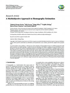
ABSTRACT In sport scenarios like football or basketball, we often deal with central views where only the central circle and some additional primitives like the central line and the central point or a touch line are visible. In this paper we first characterize, from a mathematical point of view, the set of homographies that project a given ellipse into the unit circle, next, using some extra minimal additional information like the knowledge of the position in the image of the central line and central point or a touch line we show a method to fully determine the plane homography. We present some experiments in sport scenarios to show the ability of the proposed method to properly recover the plane homography. Index Terms— Homography estimation, ellipse correspondence, camera calibration. 1. INTRODUCTION In this work we deal with the problem of camera calibration in sport event scenarios. We focus our attention on central views of the playing field where the main source of visible information is given by the projection of the central circle in the image. Moreover, some additional information can be presented as the projection of the central line, a touch line or the central point. In figure 1 we illustrate this type of scenarios.The main step in the calibration of this kind of planar view scenarios is to compute the homography from the projected playing field in the image and the reference playing field given by its actual dimensions. The usual way to compute an homography between 2 planes is to use points or lines correspondences between the image and the reference planes (see for instance [1, 2, 3, 4]). At less 4 pair correspondences are required to be able to estimate the homography, therefore this standard approach can not be used to estimate the plane homography of a central view of the playing field because the number of points and lines visible are lower than 4. We acknowledge Mediaproduci´on S.L for providing us with the real images used in this paper. This work was partially funded by the Spanish Goverment and Mediaproduci´on S.L. through the project CENIT-2007-1012 i3media and by the Spanish Goverment MICINN project MTM2010-17615.

Fig. 1. Illustration of an sport event scenario where the visible primitives are the projection of the central circle, the central line, the central point and a touch line.

In this paper we present a new closed-form solution of the homography estimation problem for central view scenarios based on a detailed mathematical analysis of the general form of the homographies transforming a given ellipse into the central circle. There are few papers in the literature which use ellipse correspondence as main source of information in image calibration. Most of them use several views to perform camera calibration. In [5] authors estimate intrinsic and extrinsic parameters using the projection of the central circle and the central line in several images. In [6] authors use the projection of a circle and right angles in 3 views to perform camera calibration. In [7] authors study the conic reconstruction problem from 2 views. In [8] authors use the projection of 2 circles in the image to perform camera calibration. In [9] authors recover 3D reconstruction from an uncalibrated image sequence of a single axis motion by fitting a conic locus to corresponding image points over multiple views. In [10], author uses the projection of a circle and the distance of 2 points to the circle to estimate the plane homography. In [11], authors compute camera intrinsic parameters using 3 views. They also estimate the plane homography using 4 point correspondences. In [12], authors use the correspondence of at least two ellipses

to perform homography estimation. In [3] authors present a technique to extract image primitives in sport event scenarios taking into account lens distortion models, they also compute the plane homography automatically identifying 2 types of scenarios corresponding to central or non-central views. As it is shown in [3], once the plane homography is computed, the lens focal distance and camera extrinsic parameters can be obtained from the homography. In [3] authors make use as a tool of the results presented in this paper but no description of the technique is presented. Concerning video processing, in [13] a technique for tracking camera motion in planar scenarios is presented. The organization of the paper is as follows: in section 2, we present the general form of an homography transforming a given ellipse into the unit circle. In section 3 and 4 we study the homography estimation using additional information like the central line and the central point or a touch line. In section 5 we present some experiments and finally in section 6 we present some conclusions. 2. GENERAL FORM OF AN HOMOGRAHY TRANSFORMING A GIVEN ELLIPSE INTO THE UNIT CIRCLE Let x ¯T A¯ x = 0 be the equation of an ellipse where A is a 3×3 symmetric matrix with eigenvalues λ1 , λ2 > 0 and λ3 < 0. Since A is symmetric, using the eigendecomposition of A we obtain an orthogonal matrix O (i.e. OT = O−1 ) given by the eigenvectors of A such that   λ1 0 0 (1) A = OT  0 λ2 0  O, 0 0 λ3 Let us introduce the following notation:   ˜ H(A) = OT  

√1 λ1

0 0

0 √1 λ2

0

0 0 √1 −λ3

  

(2)



cos z sin z 0 R(z) =  − sin z cos z 0  0 0 1  √  1 + a2 0 a  1 √ 0 B(a) =  0 2 a 0 1+a

(3)

(4)

Theorem 1 Let x ¯T A¯ x = 0 be the equation of an ellipse. We consider the 3 × 3 matrix : ˜ H = H(A) · R(α) · B(a) · R(β).

Proof: First we observe that x ¯ = Hx ¯0 . Then, replacing x ¯ by this expression in the conic formula x ¯T A¯ x = 0 we obtain the transformed ellipse equation given by x ¯0T H T AH x ¯0 = 0. On the other hand, using equations (1)-(5) we obtain the following equalities:   1 0 0 T ˜ ˜ H(A) · A · H(A) = 0 1 0  0 0 −1 

0 1 0

  0 1 0  R(z) =  0 −1 0

0 1 0

 0 0 , −1



0 1 0

  0 1 0  B(a) =  0 −1 0

0 1 0

 0 0 , −1

1 R(z)T  0 0 1 B(a)T  0 0

for any z, a ∈ R. Therefore we obtain:   1 0 0 H T AH =  0 1 0  , 0 0 −1 which means that the ellipse x ¯T A¯ x = 0 is transformed into the unit circle.  Remark 1 We point out that theorem 1 can be easily generalized to estimate the homography between any pair of ellipses. Indeed, given 2 ellipses x ¯ T A1 x ¯ = 0, x ¯ T A2 x ¯ = 0 and H1 , H2 the corresponding homographies given by (5), then we can easily show that the transformation x ¯0 = H2 H1−1 x ¯ transforms the ellipse x ¯ T A1 x ¯ = 0 into the ellipse x ¯ T A2 x ¯=0 3. COMPUTING THE PLANE HOMOGRAPHY FROM THE PROJECTION OF THE CENTRAL CIRCLE, THE CENTRAL LINE AND THE CENTRAL POINT Theorem 2 Let x ¯T A¯ x = 0 be the equation of an ellipse, a point x ¯0 inside the ellipse and a line ¯lT x ¯ = 0 passing by x ¯0 . Then there exist α, β, a ∈ R such that the transformation x ¯0 = H −1 x ¯ (where H is given by equation (5)) transforms the point x ¯0 into the point (0, 0)T and the line ¯lT x ¯ = 0 into the line x0 = 0. Proof: First we observe that by theorem 1 for any value of α, β, a ∈ R the transformation x ¯0 = H −1 x ¯ transforms the ellipse into the unit circle. On the other hand if the point x ¯0 is transformed into (0, 0) then

(5)    a cos α 0 −1 ˜  H(A) x ¯0 = sR(α)B(a)R(β)  0  = s  −a √ sin α 1 a2 + 1 

Then, for any α, β, a ∈ R the transformation x ¯0 = H −1 x ¯ T transforms the ellipse x ¯ A¯ x = 0 into the unit circle.

−1 ˜ for some s ∈ R. If we denote by x ¯00 = H(A) x ¯0 , using the above equality we obtain :

α = atan

−y00 x00

2

2



a2 =

x00 + y00



(z1 , z2 ; z3 , z4 ) =

(6)

z00 2 − x00 2 − y00 2

,

(7)

we observe that since x ¯0 is inside the ellipse, then x ¯00 is inside the unit circle and then the right part of the above equation is positive and therefore a is well defined. Finally if the line ¯lT x ¯ = 0 is transformed into the line x0 = 0 then we have : 

using the cross ratio. We recall that the cross ratio of 4 aligned points is a projective invariant defined by



1 H T ¯l = s  0  , 0

(z1 − z3 )(z2 − z4 ) (z1 − z4 )(z2 − z3 )

where z1 , z2 , z3 , z4 ∈ R are the point coordinates in any euclidean reference system defined on the line. If we compute the cross ratio of the points (0, −1), (0, 0), (0, 1) and (0, y10 ) we obtain (−1, 0; 1, y10 ) =

y10 (−1 − 1)(0 − y10 ) . = 2 (−1 − y10 )(0 − 1) 1 + y10

Next, we define an euclidean reference system in the image central line, and we denote by z−1 , z0 , z1 , zy10 ∈ R the coordinates of the projection in such reference system of the corresponding points. Therefore, since the cross ratio is a projective invariant we obtain that

for some s ∈ R. Therefore  cos β T¯ ˜ B(a)T R(α)T H(A) l = s  − sin β  , 0 

2

T¯ ˜ l, first we point out that if we write l¯0 = B(a)T R(α)T H(A) T ¯ since l x¯0 = 0 and x ¯0 is transformed into (0, 0), then (0, 0) belongs to the line ¯l0T x ¯0 = 0 and then l0 z = 0. Finally from the above equation we obtain

 β = atan

−l0 y l0 x

 (8)

which concludes the proof of the theorem  Remark 2 We notice that equations (6), (7) and (8) provide explicit formula to estimate α, a, β and then equation (5) provide a close-form solution for the homography estimation problem. 4. COMPUTING THE PLANE HOMOGRAPHY FROM THE PROJECTION OF THE CENTRAL CIRCLE, THE CENTRAL LINE AND 3 POINTS ON THE CENTRAL LINE. We assume that we know the line ¯lT x ¯ = 0, corresponding to the projection in the image of the central line (x0 = 0) and we also know a point in the image x ¯1 corresponding to the projection of a point (0, y10 ) in the central line. In practice, such point can be obtained as the interception of another line with the central line. We point out that we can compute 2 more extra point correspondences given by the interception of the unit circle and the central line, i.e. x ¯02 = (0, 1) and 0 x ¯3 = (0, −1) and the interception in the image of the ellipse and the line ¯lT x ¯ = 0. Next, we are going to show that we can compute the position of the projection of the central point

(z−1 − z1 )(z0 − zy10 ) y10 , = (z−1 , z0 ; z1 , zy10 ) = 0 1 + y1 (z−1 − zy10 )(z0 − z1 )

we notice that z−1 , z1 , zy10 are known and therefore we can estimate z0 (the projection of the central point) using the above equation and we obtain :
zy0 (z−1 − z1 ) + rz1 zy10 − z−1
z0 = 1 , (9) z−1 − z1 + r zy10 − z−1 therefore, from z0 we can recover the position in the image of the projection of the central point. Theorem 3 Let x ¯T A¯ x = 0 be the equation of an ellipse, a ¯ point x ¯1 , a line lT x ¯ = 0 passing by x ¯1 and y10 ∈ R. Using the notation explained above, if (z0 − z−1 ) · (z0 − z1 ) < 0

(10)

then there exist α, β, a ∈ R such that the transformation x ¯0 = H −1 x ¯ (where H is given by (5)) transforms the ellipse x ¯T A¯ x = 0 into the unit circle, the line ¯lT x ¯ = 0 into the central line x0 = 0, and the point x ¯1 into the point (0, y10 )T . Proof: As explained above, the knowledge of the central line in the image and an extra point x ¯1 allow us to estimate the position of the projection of the central point. Moreover, if condition (10) is satisfied, then the point z0 is located in the central line between points z−1 and z1 , therefore the projection of the central point is inside the ellipse in the image and then the statement of the theorem follows using theorem 2.  Remark 3 We point out that we can apply the above theorem in the case we know the projection in the image of the central line and the projection of another line intersecting the central line. Indeed we have just to compute the intersection point of both lines and apply the above theorem. As it is showed in the experiments, we deal with this kind of scenario very often in sport event broadcasting.

Fig. 2. Top: original Image with selected primitive points. Down: reference playing field where the original primitive points are projected using the estimated homography.

5. EXPERIMENTS We perform some experiments in simulated and real scenarios. We point out that the actual dimensions of the sport playing fields are ”a priori” known, so we can use them to built the primitives in the reference playing field we try to match with the image playing field. In figure 2 we present an experiment on a simulated scenario where we use the projection of the central circle, the central line and the central point to estimate the homograpy. In this experiment we select by hand points in the primitives to compute the primitives location. To illustrate the results we project such collection of points in the reference playing field. To measure the quality of the homography we compute the average distance between the the projected points and their associated primitive in the reference playing field. The reference playing field is given by the actual dimensions of the ”Barcelona Camp-Nou” playing field which measures 105 × 68 meters. In this case this average distance is equal to 0.067 meters which is an accurate result taking into account the playing field size and that the points are selected by hand which obviously introduce significant errors.

Fig. 3. Top: original Image with selected primitive points. Down: reference playing field where the original primitive points are projected using the estimated homography. In figure 3 we present a similar experiment in a real scenario. In this case the primitive points have been extracted in an automatic way using the technique introduced in [3]. The average distance from the projected points to their associated primitives is equal to 0.053 meters. In this case, a significant part of the error is due to lens distortion (which has not been corrected). We can observe the lens distortion phenomenon in the points of the touch lines. 6. CONCLUSIONS In this paper we present a new close-form solution for the plane homography estimation using the projection of the unit circle in the image and some minimal additional information like the projection of the central line, and the central point or a touch line. The method is based on a detailed mathematical analysis of the general form of an homography transforming a given ellipse into the unit circle. We presented some experiments which show the accuracy of the proposed method in simulated and real scenarios. As a result of this work a patent application has been filed (see [14] for more details).

7. REFERENCES [1] Chanchal Chatterjee and Vwani P. Roychowdhury, “Algorithms for coplanar camera calibration.,” Mach. Vis. Appl., vol. 12, no. 2, pp. 84–97, 2000. [2] Fl´avio Szenberg, Paulo Cezar Pinto Carvalho, and Marcelo Gattass, “Automatic camera calibration for image sequences of a football match.,” in ICAPR, Sameer Singh, Nabeel A. Murshed, and Walter G. Kropatsch, Eds. 2001, vol. 2013 of Lecture Notes in Computer Science, pp. 301–310, Springer. [3] M Alem´an-Flores, L Alvarez, L Gomez, P Henriquez, and L Mazorra, “Camera calibration in sport event scenarios,” Pattern Recognition, vol. 47, no. 1, pp. 89–95, 2014. [4] Dirk Farin, Susanne Krabbe, Peter H. N. de With, and Wolfgang Effelsberg, “Robust camera calibration for sport videos using court models.,” in Storage and Retrieval Methods and Applications for Multimedia, Minerva M. Yeung, Rainer Lienhart, and Chung-Sheng Li, Eds. 2004, vol. 5307 of SPIE Proceedings, pp. 80–91, SPIE. [5] Xianghua Ying and Hongbin Zha, “Camera calibration from a circle and a coplanar point at infinity with applications to sports scenes analyses.,” in IROS. 2007, pp. 220–225, IEEE. [6] Huang Zhong, Fei Mai, and Y. S. Hung, “Camera calibration using circle and right angles.,” in ICPR (1). 2006, pp. 646–649, IEEE Computer Society. [7] Long Quan, “Conic reconstruction and correspondence from two views.,” IEEE Trans. Pattern Anal. Mach. Intell., vol. 18, no. 2, pp. 151–160, 1996. [8] Qian Chen, Haiyuan Wu, and Toshikazu Wada, “Camera calibration with two arbitrary coplanar circles.,” in ECCV (3), Tom´as Pajdla and Jiri Matas, Eds. 2004, vol. 3023 of Lecture Notes in Computer Science, pp. 521– 532, Springer. [9] Guang Jiang, Hung-Tat Tsui, Long Quan, and Andrew Zisserman, “Geometry of single axis motions using conic fitting.,” IEEE Trans. Pattern Anal. Mach. Intell., vol. 25, no. 10, pp. 1343–1348, 2003. [10] Feng Guo, “Plane rectification using a circle and points from a single view.,” in ICPR (2). 2006, pp. 9–12, IEEE Computer Society. [11] Qihe Li and Yupin Luo, “Automatic camera calibration for images of soccer match.,” in International Conference on Computational Intelligence, Ali Okatan, Ed. 2004, pp. 482–485, International Computational Intelligence Society.

[12] Kannala J., Salo M, and Heikkil¨a J., “Algorithms for computing a planar homography from conics in correspondence,” in Proc. the 16th British Machine Vision Conference (BMVC 2006), Edinburgh, UK, 2006, vol. 1, pp. 77–86. [13] Luis Alvarez, Luis Gomez, Pedro Henriquez, and Javier S´anchez, “Real-time camera motion tracking in planar view scenarios,” Journal of Real-Time Image Processing, pp. 1–13, 2013. [14] L. Alvarez and V. Caselles, “Calibration method for a tv and video camera,” Feb. 2011, EP Patent Number : EP2287806 A1.