Ellipsoid ART and ARTMAP for incremental unsupervised ... - CiteSeerX

header for SPIE use

Ellipsoid ART and ARTMAP for incremental unsupervised and supervised Learning Georgios C. Anagnostopoulos* and Michael Georgiopoulos** School of Electrical Engineering & Computer Science University of Central Florida, Orlando, Florida ABSTRACT We introduce Ellipsoid-ART (EA) and Ellipsoid-ARTMAP (EAM) as a generalization of Hyper-sphere ART and Hypersphere-ARTMAP respectively. Our novel architectures are based on ideas rooted in Fuzzy-ART (FA) and FuzzyARTMAP (FAM). While FA/FAM summarize input data using hyper-rectangles, EA/EAM utilize hyper-ellipsoids for the same purpose. Due to their learning rules, EA and EAM share virtually all properties and characteristics of their FA/FAM counterparts. Preliminary experimentation implies that EA and EAM are to be viewed as good alternatives to FA and FAM for data clustering and classification tasks. Extensive pseudo-code is provided in the appendices for computationally efficient implementations of EA/EAM training and performance phases. Keywords: adaptive resonance theory, self-organization, clustering, classification, Fuzzy ART, Fuzzy ARTMAP.

1. INTRODUCTION Fuzzy-ART1 (FA) and Fuzzy-ARTMAP2 (FAM) are two neural network architectures based on the adaptive resonance theory that addresses Grossberg's stability-plasticity dilemma3. While FA can be used for clustering of data, FAM is capable of forming associations between clusters of two different spaces and, as a special case, can be used as a classifier too. In this paper we will focus more on the classification capabilities of FAM rather than its ability to associate clusters. Therefore, when we refer to FAM, we will mean the FAM architecture customized for classification tasks. An important feature of FA/FAM is the ability to undergo both batch (off-line) and incremental (on-line) learning. In off-line learning, a set of training patterns is repeatedly presented until the completion of the learning task at hand. In contrast, during on-line learning, the networks’ structure is being altered as necessary to explain the existence of new patterns as they become available. Under a special modus operandi called fast learning, a particularly interesting property of these networks is that they complete their learning in a finite number of steps. In other words, their training procedure converges fast to a stable state in a finite number of list presentations (epochs). This is in contrast, for example, to feed-forward neural networks, which use the Backprop algorithm for their training and only asymptotically reach a stable state. Moreover, once fast learning has reached its completion FAM achieves a 100% correct classification on its training set. In order to perform their learning task (clustering for FA and classification for FAM), both architectures group their input data into clusters (FA categories or simply categories). FA forms its categories from unlabeled input patterns via an unsupervised learning scheme, while in FAM categories are formed in a supervised manner and consist of input patterns bearing the same class label. Note that, in FAM many categories might describe a single class of patterns and therefore share a common class label. FA and FAM can be thought of as networks that during training perform compression of their inputs by substituting single patterns with clusters. The forming of clusters is achieved via a self-organizing scheme; FA/FAM perform their tasks without optimizing a specific objective function. Both of them process real-valued, vector-valued data; both cannot cope with data featuring missing attribute values. Also, FA and FAM work especially well, when the data is binary-valued. Furthermore, both of the networks require a preprocessing stage, where either input pattern normalization or complement coding is used to prevent category proliferation. While input data normalization causes a loss of vector-length information, complement coding normalizes input vectors and preserves their amplitude information. Another interesting aspect of the two architectures is that due to the internal structure, it is easy to explain the networks’ outputs, such as why a particular pattern was selected by a category. This is not the case, for example, with feed-forward neural architectures, where it is significantly difficult to explain why an input x generates a certain output y. A key element in the learning process of the two architectures is a non-typical pattern detection mechanism that is capable of identifying patterns, whose presence is not explained by the already developed (via learning) categories within the networks. Thus, during training phase, a pattern that does not fit the characteristics of already existing categories will initiate the creation of a new category. Aside from FA/FAM’s advantages, criticism4 has been voiced on the lack of a smoothing operation during learning that would ameliorate *[email protected]; phone 1 407 371-7192; fax 1 407 371-7152; http://www.seecs.ucf.edu/; School of EECS, University of Central Florida, 4000 Central Florida Blvd., Orlando, FL 32816; **[email protected]; phone 1 407 823-5338; fax 1 407 823-5835; http://www.seecs.ucf.edu/; School of EECS, University of Central Florida, 4000 Central Florida Blvd., Orlando, FL 32816.

the effects of noise present in the data. The architectures use hard-competitive learning to form their categories, hence, overfitting becomes an issue. On the next page we summarize in a table the main characteristics of FA/FAM. The interested reader might find properties of learning for FA and FAM in other references5,6. Due to space limitations, we assume that the reader already possesses a rudimentary background in FA and FAM.

Characteristics of FA/FAM Capable of both off-line and on-line learning. Capable of fast, finite, stable learning. Feature an outlier detection mechanism. Network behavior upon presentation of a pattern is easily explained. Are sensitive to noise and prone to over-fitting, because they do not feature a noise removal mechanism. Table 1: Main characteristic of FA/FAM learning.

The organization of this paper is as follows: first we state the motivation behind developing EA and EAM as extensions to FA and FAM respectively and continue with the description of the novel architectures/algorithms. Later in this paper, we present some illustrative experimental results, which compare EAM to the original FAM, and finally we state our conclusions. Extensive pseudo-code is provided for a computationally efficient software implementation of both EA and EAM training (Appendix A) and performance (Appendix B) phases. As a general comment, you will notice that our intent is to highlight some algorithmic elements of the architectures described in this paper, rather than focusing on their architectural nature. In other words, in this paper we emphasize the view of FA/FAM and EA/EAM as clustering and classification algorithms respectively.

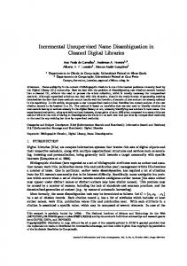
2. ELLIPSOID-ART & ELLISPOID-ARTMAP FA and FAM utilize hyper-rectangles for category representation, which works especially well for patterns, whose attributes take quantized values (for example, patterns with binary valued-features). Note, that if M is the dimensionality of the input space, then each FA category requires 2M memory units (floating point numbers, for example). When it comes to clustering problems, depending on the distribution of input space patterns, hyper-rectangles are not always the ideal shape to represent clusters7. Furthermore, regarding classification tasks, due to the fact that both algorithms utilize city-block (L1) distances, it can be shown that decision boundaries created by FAM are piece-wise linear. Based on these facts as a motivating point, Gaussian-ART7 (GA) and Gaussian-ARTMAP7 (GAM) addressed this issue successfully using hyper-ellipsoids for the geometric representation of categories utilizing also 2M memory units per category. A characteristic of GA/GAM is that their hyper-ellipsoids are constrained to have their axes parallel to the corresponding ones of the input space’s coordinate system. Although there are several similarities between GA/GAM and FA/FAM, the former ones do not feature an appealing property of the latter ones, which is to complete the off-line training phase in a finite number of list presentations under fast learning conditions (learning rate γ equals 1). Hypersphere-ART8 (HA) and Hypersphere-ARTMAP8 (HAM) were the first neural network architectures to employ shapes (hyper-spheres) other than hyper-rectangles for category description, while maintaining the major (if not all) properties of FA and FAM. In HA/HAM, hyper-spheres require M+1 memory units per category and are capable of forming more complex decision boundaries than FA/FAM. In this paper we present EA and EAM, which are a successful attempt of using hyper-ellipsoids as category representations with 2M+1 memory units per category, while simultaneously retaining virtually all of the properties and characteristics of FA and FAM respectively. The new architectures essentially extend the ideas first presented in HA/HAM. To guarantee the inheritance of FA/FAM properties, during the training phase EA categories have to be updated in such a manner so that they comply to the following two constraints: i) the hyper-ellipsoids must maintain a constant ratio µ between the lengths of their major axis and their remaining axes and ii) the hyper-ellipsoids must also maintain constant the direction of their major axis once it is set. Despite the above limitations, EA categories can have arbitrary orientations in the input space in order to capture the characteristics of the data. An EA category j corresponds to each node in the EA module’s F2 layer and is described by its template vector wj=[mj dj Rj], where mj is the center of the hyper-ellipsoid, dj is called the category’s direction vector, which coincides with the direction of the hyper-ellipsoid’s major axis, and Rj is called the category’s radius, which equals half of the major axis’ length. The category’s size s(wj) is defined as the major axis’ full length and equals 2Rj. A comparison between a 2-dimensional FA and EA category is given in Figure 1.

vj dj µ Rj

mj

s ( w j)

R j = s ( w j)/2

uj

Figure 1: 2-dimensional FA and EA categories with template elements. EA/EAM geometry revolves around the use of weighted Euclidian distances, rather than the city-block (L1) distance of FA/FAM. Distances of patterns from an EA category j depend on the category’s shape matrix Cj defined as

Cj =

C Tj

[

 1 T I − (1 − µ 2 )d j d j  = µ 2  I 

]

if d j ≠ 0

.

(1)

if d j = 0

In the above expression, µ is the ratio of the hyper-ellipsoid’s major axis length over the length of each other minor axes. Also, all vectors are arranged in columns and the T-exponent signifies the transpose of the quantity it is applied upon. Note, that for EA categories that encode a single pattern, dj is defined to equal the zero vector 0 and the shape matrix Cj is defined to equal the identity matrix I. In general, the distance of an input pattern x from an EA category j is given as dis(x | w j ) = max x − m j 

Cj

, R j  − R j . 

(2)

where we define x−m j

Cj

(

= x −m j

)T C j (x − m j ).

(3)

Instead of explicitly forming the shape matrix Cj, using Equation 1 we can calculate the distance of a pattern x from the center mj of a category j with shape matrix Cj according to

x−mj

Cj

1  = µ  

x−mj

2 2

[

T 2 − (1 − µ ) d j (x − m j )

x−mj

]

2

if d j ≠ 0

.

(4)

if d j = 0

2

In Eq. 4, ||⋅||2 denotes the usual Euclidian (L2) norm of its vector argument. Based on Equation 2, we define the representation region of an EA category j as the set of all points of the input space satisfying dis(x | w j ) = 0

⇒

x−m j

Cj

2 ≤ Rj .

(5)

In Figure 1 the shaded areas correspond to the representation regions of the categories involved. The shape of the representation regions in EA/EAM depends on the order, according to which patterns are being presented during training, and the EA/EAM network parameters. EA/EAM feature 4 network parameters: D (which plays the role of M in FA/FAM), the (common for all categories) ratio µ∈(0,1] of minor-to-major axes lengths, the vigilance parameter ρ∈[0,1] and the choice

parameter a>0 (the value a=0 is valid only for EA). In the case of EAM for classification tasks, these parameters will refer to the ones of its ARTa module, since the ones of ARTb are of no practical interest. The ARTa module corresponds to the input domain and ARTb to the output domain of EAM. When EAM is used as a classifier the output domain coincides with the set of class labels pertinent to the classification problem. As was the case with HA/HAM8, the definition of the category match function (CMF) ρ(wj|x) and the category choice function (CCF) T(wj|x), also known as bottom-up input or activation function, for an EA category j is based on the homologous expressions valid for FA categories:

ρ (w j | x) =

T (w j | x) =

D − s(w j ) − dis(x, w j ) D D − s (w j ) − dis(x, w j ) D − s (w j ) + a

⇒

⇒

 R j + maxR j , x − m j  ρ (w j | x) = 1 − D  D − R j − max R j , x − m j  T (w j | x) = D − 2R j + a

Cj

  

Cj

.

  

(6)

.

(7)

Uncommitted nodes in EA/EAM feature a constant CMF value of ρu=1 and a constant CCF value of Tu=D/(2D+a) for all patterns of the input space. Furthermore, uncommitted nodes do not correspond to any category; they just represent the “blank” memory of the networks. As a reminder, the CMF value of a category is used for its comparison to the vigilance parameter, when performing the vigilance test (VT). Also, the category’s CCF value is used for its comparison to the CCF value Tu of the uncommitted node, when performing the commitment test (CT), and to determine a winning category during node competition in the F2 layer for an input pattern. Care should be taken, when choosing a value for D. To guarantee that the CMF’s and the CCF’s value for all categories and for all possible input patterns lies in the interval [0,1], D should be selected at least equal to the maximum possible Euclidian distance between patterns of the input space (Euclidian input space diameter) in consideration, that is, D ≥ max x p − x q p,q

2

.

(8)

EA/EAM training phases are identical to the ones of FA/FAM. Upon presentation of a new training pattern all committed nodes in the F2 layer (that correspond to existing categories) are initially assumed to belong to a candidate set S, whose members are eligible to encode the pattern. As a first step, all members of S undergo the VT, which removes from S all categories with CMF value less than ρ. Next, the remaining members of S (if any) compete with each other in terms of CCF values. An uncommitted node also participates in the competition, which constitutes the CT. Categories with CCF value less than Tu are filtered out of S. If no category passes both the VT and the CT (thus, S is empty), an uncommitted node becomes committed and forms a new category that encodes the new pattern. In the case of EA, if S is non-empty after the VT and CT, the category featuring the highest CCF value is allowed to encode the pattern. On the other hand, in the case of EAM, the course of action depends on the comparison of labels between the pattern and the chosen category. If the pattern and the chosen category share a common label, then the category is allowed to encode the pattern. Otherwise, if there’s label mismatch, match tracking2 (MT) is performed. EA categories encode training patterns by updating their templates. During training, EA categories can only grow in size and therefore can never be destroyed. The learning rules of EA/EAM resemble the ones of HA/HAM8 and are depicted below. The learning rate is denoted as γ∈(0,1]; γ=1 corresponds to fast learning. Also, x(2) denotes the second pattern to be encoded in category j. = R old R new j j +

= m old m new j j

γ  old  maxR old j , x−mj 2 

  old  min R old j , x−mj γ  + 1− 2 x − m old j  C  old j

C old j

C old j

 old   − R j  .  

(9)

    x − m old . j   

(

)

(10)

x ( 2) − m j

dj =

x (2) − m j

.

(11)

2

Equation 9 and 10 imply that, when a training pattern is already located inside the representation region of category j, no updates will take place for this category. Figure 2 provides a 2-dimensional illustration of a comparison between FA and EA category updates. In case of a category update, due to the learning rules in Equations 9 through 11, the category’s new representation region can be shown to be the minimum hyper-volume hyper-ellipsoid that simultaneously contains both the old representation region and the new pattern to be encoded (provided that the new pattern is not the second one to be encoded by the category). Notice, that once the EA category’s direction vector dj has been set, it remains constant during future updates. Notice, also that the boundaries of the two ellipsoids Eold and Enew touch only at one point, t(x,wjold).

E new v j old

v jnew

E old

d j old mj u j old

u jnew

Rj R new

x

m jnew

t ( x , w j old)

R old

d jnew

old

old

R jnew

x

Figure 2: Category update assuming fast learning in FA/FAM and EA/EAM in 2 dimensions.

A typical lifecycle of an EA category under fast learning assumptions is depicted in Figure 3. When category j is first created upon presentation of pattern x1, its center mj coincides with x1, its direction vector is dj=0 and its radius is Rj=0. Assuming that category j is eligible to encode pattern x2, the category’s representation region expands into an ellipse with its center mj amidst x1 and x2, Rj equal to the Euclidian distance between x1 and x2 and, finally, dj is set equal to the unit Euclidian-length vector along the direction of x2-x1. Assuming that category j is also eligible to encode x3, the representation region expands enough to include the previous representation region and the new pattern, while maintaining constant its relative form (constant ratio µ of minor axis length over major axis length) and constant direction (constant direction vector dj).

x3

x3

x3

x2

x2 mj

m j= x 1

x1

dj

x2 mj

dj

x1

Figure 3: Lifecycle of an EA category in 2 dimensions under fast learning.

The performance phases of EA/EAM are also identical to the ones of FA/FAM. To force EAM to classify a test pattern to one of the existing classes, the vigilance ρ has to be set equal to 0 and uncommitted nodes have to be excluded from node competitions, thus, no CT must be performed. An interesting fact regarding EAM is that, if it is trained using ρ=1 and then

is being used as a classifier with ρ=0 without requiring the CT during performance, EAM becomes equivalent to the L2-norm (Euclidian) 1-Nearest Neighbor classifier9. Furthermore, if µ=1 EA/EAM become equivalent to HA/HAM, which justifies our statement, that EA/EAM are generalizations of HA/HAM.

Figure 4: Decision boundaries example for FAM and EAM. The advantage of EAM in certain classification tasks can be attributed also on the fact that it can create decision boundaries that are non-linear, in contrast to FAM, which composes only piece-wise linear boundaries. An example of this fact is shown in Figure 4, where FAM and EAM have to separate two classes with no overlap on the plane. Points marked as asterisks stand for training patterns. Black regions signify points in the plane classified as class 0 and white ones as class 1. The gray areas constitute points deemed by the classifiers as non-typical of the training data via the VT and/or the CT. Also, each rectangle corresponds to a FA category and each ellipse to an EA category. As you may have observed, the number of categories created through training differs between Figures 4a, 4b and 4c, 4d. This has been achieved by using different values for the network parameters.

3. EXPERIMENTAL RESULTS In general, an objective comparison of clustering algorithms is difficult to be achieved, thus, we will not attempt to directly compare EA with FA. However, we can show the potential of the EA/EAM family by comparing EAM with FAM on the basis of classification performance. We chose a simple, artificial classification example for our purposes, namely the Circlein-a-Square problem. It has been used in the past as a benchmark problem in the DARPA artificial neural network technology (ANNT) program10. A circle of radius R = 1 / 2π is inscribed in the unit square, so that its interior covers exactly half of the unit square’s surface. The classifiers have to learn how to distinguish points inside the circle (class label 1) from points outside it (class label 0). Ten training sets have been created drawing samples from each class with equal probability. Each set contains a multiple of 10 worth of training patterns: the first set contains 10, the second 20, etc. Also, a test set was created with 10200 equally spaced labeled patterns that form a grid of points inside the unit square. Both classifiers were trained until completion of fast learning using the same order of training patterns. A variety of network parameter values were used for both FAM and EAM. The classification performance results are illustrated in Table 2 below.

Training set cardinality 10 20 30 40 50 60 70 80 90 100

FAM EAM EAM EAM pattern %performance %performance %improvement advantage 66.405254 65.101461 -1.303793 -13300 72.865405 74.875012 2.009607 20500 86.383688 85.677875 -0.705813 -7200 88.167827 88.354083 0.186256 1900 89.716694 89.873542 0.156848 1600 84.158416 84.089795 -0.068621 -700 90.167631 90.079404 -0.088227 -900 89.83433 91.412607 1.578277 16100 88.971669 89.795118 0.823449 8400 91.22635 91.657681 0.431331 4400

Table 2: Comparison of classification performance between FAM and EAM on the Circle-in-a-Square Problem.

Columns 2 and 3 contain the percent correct classification rate of FAM and EAM respectively. Column 4 depicts the difference of percent correct classification between EAM and FAM. Finally, column 5 shows the number of test patterns that corresponds to the difference of percent correct classification between EAM and FAM (value in Column 4). Evidently, in 6 out of 10 cases EAM slightly outperforms FAM with a maximum difference of 2%. We are currently in the process of performing additional experiments using machine learning databases to study the classification performance of EAM with respect to FAM and to other classification algorithms.

4. CONCLUSIONS In this paper we have presented two novel neural network architectures, namely Ellipsoid-ART and Ellipsoid-ARTMAP for clustering and classification tasks respectively. These architectures are based on principals and key ideas of Fuzzy-ART and Fuzzy-ARTMAP and therefore inherit they learning properties: they are capable of batch and on-line learning, exhibit fast, stable, finite learning and they both are equipped with an outlier detection mechanism. Moreover, they can be regarded as generalizations of Hypersphere-ART and Hypersphere-ARTMAP. Both of them use hyper-ellipsoids as the means to summarize input data, in contrast to FA/FAM, which use hyper-rectangles. Therefore, they are not constrained to creating only piece-wise linear decision boundaries. Finally, we have demonstrated with limited experimental results that EA and EAM can be considered worthy alternatives to FA and FAM.

REFERENCES 1.

G.A. Carpenter, S. Grossberg and D.B. Rosen, “Fuzzy ART: Fast stable learning and categorization of analog patterns by an adaptive resonance system”, Neural Networks, 4(6), pp. 759-771, 1991. 2. G.A. Carpenter, S. Grossberg, N. Markuzon, J.H. Reynolds and D.B. Rosen, “Fuzzy ARTMAP: A Neural Network Architecture for Incremental Supervised Learning of Analog Multidimensional Maps”, IEEE Transaction on Neural Networks, 3(5), pp. 698-713, 1992. 3. S. Grossberg, “Adaptive pattern recognition and universal encoding II: Feedback, expectation, olfaction, and illusions”, Biological Cybernetics, 23, pp. 187-202, 1976. 4. A. Baraldi and P. Blonda, “A Survey of Fuzzy Clustering Algorithms for Pattern Recognition – Part II”, IEEE Transactions on Systems, Man and Cybernetics, Part B: Cybernetics, 29(6), pp. 786-801, December 1999. 5. J. Huang, M. Georgiopoulos and G.L. Heileman, “Fuzzy ART Properties”, Neural Networks, 8(2), pp. 203-213, 1995. 6. M. Georgiopoulos, H. Fernlund, G. Bebis and G.L. Heileman, “Order of Search in Fuzzy ART and Fuzzy ARTMAP: Effect of the choice parameter”, Neural Networks, 9(9), pp. 1541-1559, 1996. 7. J.R. Williamson, “Gaussian ARTMAP: A Neural Network for Fast Incremental Learning of Noisy Multidimensional Maps”, Neural Networks, 9(5), pp. 881-897, 1996. 8. G.C. Anagnostopoulos and M. Georgiopoulos, “Hypersphere ART and ARTMAP for Unsupervised and Supervised, Incremental Learning”, Proceedings of the IEEE-INNS-ENNS International Joint Conference on Neural Networks, 6, pp. 59-64, Como, Italy, 2000. 9. G. Wilensky, “Analysis of neural network issues: Scaling, enhanced nodal processing, comparison with standard classification”, DARPA Neural Network Program Review, October 29-30, 1990. 10. R.O. Duda and P.E.Hart, “Pattern classification and scene analysis”, New York, Wiley, 1973.

APPENDIX A The algorithm below implements EA/EAM (EAM for classification) off-line training phase assuming fast learning. N is the number of existing categories in EA/EAM , P is the number of training patterns, M is the dimensionality of the input patterns, S is the candidate set and {D,ρ, a} are the network parameters. Lines starting with double back-slashes (“//”) represent comments. // Initialization D , N :=0 2D + a Set the Candidate Set to empty, i.e. S :=∅ . Set const1:=Mρ, const2:=D+a , Tu :=

// List presentation (epoch) loop. Until no more categories have been created or updated, do { // Pattern loop. For each training pattern xp p:=1..P { // Calculate the category match function values. For each category j:=1..N {

Calculate dis(x p , m j ) := x p − m j

CJ

Calculate dis(x p , w j ) := dis(x p , m j ) − R j // If xp is outside the category’s representation region If dis(x p , w j ) > 0 {

Calculate the scaled vigilance ρ * (w j | x p ) = Dρ (w j | x p ) := D − s (w j ) − dis (x p , w j ) // Perform a test equivalent to VT. If ρ * (w j | x p ) ≥ const1 , then include category j in S.

} Else, if dis(x p , w j ) ≤ 0 {

// Pattern xp lies inside the representation region of category j,

// therefore it is guaranteed that j passes the VT for xp. Include category j in S. Set dis(x p , w j ) := 0 } } // End of category loop // If at least one existing category passed the VT If S ≠ ∅ { // Calculate the category choice function values. For each category j in S Calculate the CCF value T (w j | x p ) :=

ρ * (w j | x p ) const 2 − s (w j )

// Find the category with the maximum category choice function value. Determine the maximum value Tmax of T(wj |xp) from the categories in S. Simultaneously, find the category with the smallest index j, for which T(wj |xp)=Tmax. Assume that it is category k. // Perform the CT on category k. If Tmax 0 {

Calculate the scaled vigilance ρ * (w j | x p ) = Dρ (w j | x p ) := D − s (w j ) − dis (x p , w j ) // Perform a test equivalent to VT. If ρ * (x p | w j ) ≥ const1 , then include category j in S.

} Else, if dis(x p , w j ) ≤ 0 {

// Pattern xp lies inside the representation region of category j, // therefore it is guaranteed that j passes the VT for xp. Include category j in S. Set dis(x p , w j ) := 0

} } // End of category loop // If at least one existing category passed the VT If S ≠ ∅ { // Calculate the category choice function values. For each category j in S Calculate the CCF value T (w j | x p ) :=

ρ * (w j | x p ) const 2 − s (w j )

// Find the category with the maximum category choice function value Determine the maximum value Tmax of T(wj |xp) from the categories in S. Simultaneously, find the category with the smallest index j, for which T(wj |xp)=Tmax. Assume that it is category k. Set J:=k.

If CT-option is TRUE { // The uncommitted nodes participate in the node competition. // Perform the CT for category k. If Tmax