Incremental Techniques for Mining Dynamic and ... - CiteSeerX

Incremental Techniques for Mining Dynamic and Distributed Databases Matthew Eric Otey† Adriano Veloso†‡ Chao Wang† Srinivasan Parthasarathy† Wagner Meira Jr.‡ †

Computer and Information Science Department The Ohio-State University Computer Science Department Universidade Federal de Minas Gerais ‡

Contact:

[email protected]

Abstract Traditional methods for data mining typically make the assumptions that the data is centralized and static. These assumptions are no longer tenable. Such methods impose excessive communication overhead when data is distributed. Also, they waste computational and I/O resources when data is dynamic. In this paper we present what we believe to be the first data mining approach that overcomes all these assumptions. In fact, we consider a broader scenario in which the data is continuously updated and stored at geographically different locations. This scenario imposes several challenges to data mining, especially those concerning performance and interactivity. Our approach makes use of parallel and incremental techniques to generate frequent itemsets even in the presence of data updates without examining the entire database. It also imposes minimal communication overhead when mining distributed databases. Further, our approach is capable of generating both local models (in which each site has a summary of its own database) as well as the global model of frequent itemsets (in which all sites have a summary of the entire database). This ability permits our approach not only to generate frequent itemsets, but also high-contrast frequent itemsets, from which users can know those itemsets that have their supports unevenly distributed among the distributed databases.

1 Introduction Advances in computing and networking technologies have resulted in large distributed and dynamic sources of data. A classic example of such a scenario is found in the databases of large national and multinational corporations. Such databases/warehouses are often composed of disjoint databases located at geographically different sites. Each database is continuously being updated with new data as transactions transpire. The update rate and ancillary properties may be unique to a given site. A user may be interested in mining such databases in a variety of ways. They may desire to generate a global model of the database, thus the sites must exchange some information about their local models. However, the information exchange must be made in a way that minimizes the communication overhead. The frequency at which the global model is updated may vary from the frequency with each local model is updated. Furthermore, in such a distributed scenario, the user may be interested in not only knowing the global data mining model, but also the differences (or contrasts) between the local models. Analyzing these large distributed and potentially dynamic databases requires non-trivial data mining approaches, approaches that make proper use of the distributed resources, minimize communication requirements, adapt to user interaction requirements and minimize/eliminate work replication. In this paper we present an efficient approach for finding the model of frequent itemsets when the data is both distributed and dynamic. Also, our approach is able to generate the model of high-contrast frequent itemsets, from which the user can identify interesting patterns that disambiguate among local databases. The main contributions of our paper can be summarized as follows: • An cluster of SMP sensitive parallel algorithm based on the Z IG Z AG incremental mining approach[13]. This algorithm is used to update the model at a local site. • A distributed incremental mining algorithm that minimizes the communication costs for mining over a wide area network or grid-space. This algorithm is used to update the global model. • Novel interactive extensions for computing high contrast frequent itemsets, and query response time sensitive (approximate) parallel and distributed algorithms. • Extensive experimentation and validation on real databases. The rest of the paper is organized as follows. In Section 2 we highlight background and related work. Section 3 we describe the algorithms and novel interactive extensions. Section 4 validates the algorithms and proposed work through extensive experimental results. Concluding remarks are made in Section 5.

2 Background and Related Work The frequent itemset mining task can be stated as follows: Let I be a set of distinct attributes, also called items. Let D be a database of transactions, where each transaction has a unique

identifier (tid) and contains a set of items. A set of items is called an itemset where for each nonnegative integer k, an itemset with exactly k items is called a k-itemset. The tidset of an itemset C corresponds to the set of all transaction identifiers (tids) where the itemset C occurs. The support count of C, is the number of transactions of D in which it occurs as a subset. Similarly, the support of C, denoted by σ(C), is the percentage of transactions of D in which it occurs as a subset. The itemsets that meet a user specified minimum support are referred to as frequent itemsets. A frequent itemset is maximal if it is not subset of any other frequent itemset.

2.1 Mining Distributed Databases A common approach for mining distributed databases is the centralized one, in which all data is moved to a single central location and then mined. Another common approach is the local one, where models are built locally in each site, and then moved to a common location where they are combined. The later approach is the quickest but often the least accurate, while the former approach is more accurate but generally quite expensive in terms of time required. In the search for accurate and efficient solutions, some intermediate approaches have been proposed [1, 3, 6, 15]. In [1] three distributed mining approaches were proposed. The C OUNT D ISTRIBUTION algorithm is a simple distributed implementation of A PRIORI [2]. All sites generate the entire set of candidates, and each site can thus independently get local support counts from its partition. At each iteration the algorithm does a sum reduction operation to obtain the global support counts by exchanging local support counts with all other sites. Since only the support counts are exchanged among the sites, the communication overhead is reduced. However, it performs one round of communication per iteration (note that synchronization is implicit in communication). The DATA D ISTRIBUTION algorithm generates disjoint candidate sets on each site. However, to generate the global support counts, each site has to scan the entire database (its local partition and all remote ones) in all iterations of the algorithm. Hence this approach suffers from high I/O overhead. The C ANDIDATE D ISTRIBUTION algorithm partitions the candidates during each iteration, so that each site can generate disjoint candidates independently of the other sites, but it still requires one round of communication per iteration. In [15] two distributed algorithms were presented, PAR E CLAT and PAR M AX E CLAT. Both algorithms are based on the concept of equivalence classes. Each equivalence class corresponds to a subtree in the search space for frequent itemsets, and they can be processed asynchronously on each site. PAR E CLAT outperforms DATA, C OUNT, and C ANDIDATE D ISTRIBUTION algorithms for more than one order of magnitude. PAR M AX E CLAT outperforms PAR E CLAT, but it searches only the maximal frequent itemsets, instead of all frequent itemsets. These techniques are devised to scale up a given algorithm (e.g., A PRIORI, E CLAT, etc.).

Data is distributed (or in some cases, replicated) among different sites and a data mining algorithm is executed in parallel on each site. These approaches do not take into account the possible distributed nature of the data. Some assume a high-speed network environment and perform excessive communication operations. These approaches are not efficient when the databases are geographically distributed.

2.2 Mining Dynamic Databases Some recent effort has been devoted to the problem of incrementally mining frequent itemsets [11, 12, 13, 4, 5, 9] in dynamic databases. Some of these algorithms cope with the problem of determining when to update the current model of frequent itemsets, while others update the model after an arbitrary number of updates [13]. To decide when to update, Lee and Cheung [11] propose the D ELI algorithm, which uses statistical sampling methods to determine when the current model is outdated. A similar approach proposed by Ganti et al [9] monitors changes in the data stream. An efficient incremental algorithm, called ULI, was proposed by Thommas [12] et al. ULI strives to reduce the I/O requirements for updating the set of frequent itemsets by maintaining the previous frequent itemsets and the negative border [?] along with their support counts. The whole database is scanned just once, but the incremental database must be scanned as many times as the size of the longest frequent itemset.

3 Parallel and Distributed Incremental Mining In this section we will describe our parallel and distributed incremental mining algorithms. Specifically, the idea is that within a local domain one can resort to parallel mining approaches (either within a node or within a cluster) and across domains one can resort to distributed mining approaches (across clusters). The key distinction between the two scenarios being the cost of communication. Below we first give the problem statement.

3.1 Problem Definition Using D as a starting point, a set of new transactions d+ is added and a set of old transactions

d− is removed, forming the dynamic database ∆ (i.e., ∆ = (D ∪ d+ ) − d− ). Let sD be the minimum support used when mining D, and FD be the set of frequent itemsets obtained. Let Π be the information kept from the current mining that will be used in the next incremental mining operation. In our case, Π consists of FD (i.e., all frequent itemsets, along with their support counts, in D). An itemset C is frequent in ∆ if its support is no less than s ∆ . Note

that an itemset C not frequent in D, may become a frequent itemset in ∆ (defined as emerged itemset). If a frequent itemset in D remains frequent in ∆ it is called a retained itemset.

The database ∆ can be divided into n partitions, δ1 , δ2 , ..., δn . Each partition δi is assigned

to a site Si . Let C.sup and C.supi be the respective support counts of C in ∆ and δi . We will call C.sup the global support count of C, and C.supi the local support count of C in δi . For a given minimum support s∆ , C is global frequent if C.sup ≥ s∆ × | ∆ |; correspondingly, C is local frequent at δi , if C.supi ≥ s∆ × | δi |. C is a high-contrast frequent itemset if it is global frequent, and if its local support counts differ meaningfully accross each partition δ i . The set of all maximal global frequent itemsets is denoted as global MFI∆ , and the set of maximal local frequent itemsets at δi is denoted as MFIδi . The task of mining frequent itemsets in distributed and dynamic databases is to find F∆ (i.e., all global frequent itemsets in ∆), with respect to a minimum support s∆ and, more importantly, using Π and minimizing access to D (the original

database) to enhance the algorithm performance.

3.2 The Z IG Z AG Incremental Algorithm In this section we briefly describe the Z IG Z AG [13] incremental algorithm (sequential) that we use as a basis for our parallel and distributed incremental algorithms. Almost all algorithms for mining frequent itemsets use the same procedure − first a set of candidates is generated, the infrequent ones are pruned, and only the frequent ones are used to generate the next set of candidates. Clearly, an important issue in this task is to reduce the number of candidates generated. An interesting approach to reduce the number of candidates is to first find MFI∆ . Once MFI∆ is found, it is straightforward to obtain all frequent itemsets (and their support counts) in a single database scan, without generating infrequent (and unnecessary) candidates. This approach works because the downward closure property (all subsets of a frequent itemset must be frequent). The number of candidates generated to find MFI ∆ is much smaller than the number of candidates generated to directly find all frequent itemsets. The maximal frequent itemsets has been successfully used in several data mining tasks, including incremental mining of dynamic databases [13, 14]. An efficient incremental algorithm for mining dynamic databases named Z IG Z AG was proposed in [13]. The main idea is to incrementally compute MFI∆ using the previous knowledge Π. This avoids the generation and testing of many unnecessary candidates. Having MFI ∆ is sufficient to know which itemsets are frequent; their exact support are then obtained by examining d+ , d− and using Π, or, where this is not possible, by examining ∆. Z IG Z AG employs a backtracking search to find MFI∆ . Backtracking algorithms are useful for many combinatorial problems where the solution can be represented as a set I = {i 0 , i1 , ...}, where each ij is chosen from a finite possible set, Pj . Initially I is empty; it is extended one item at a time as the search space is traversed. The length of I is the same as the depth of the corresponding node in the search tree. Given a k-candidate itemset, Ik = {i0 , i1 , ..., ik−1 }, the

possible values for the next item ik comes from a subset Rk ⊆ Pk called the combine set. If y ∈ Pk − Rk , then nodes in the subtree with root node Ik = {i0 , i1 , ..., ik−1 , y} will not be considered by the backtracking algorithm. Each iteration of the algorithm tries to extend I k with every item

x in the combine set Rk . An extension is valid if the resulting itemset Ik+1 is frequent and is not a subset of any already known maximal frequent itemset. The next step is to extract the new possible set of extensions, Pk+1 , which consists only of items in Rk that follow x. The new combine set, Rk+1 , consists of those items in the possible set that produce a frequent itemset when used to extend Ik+1 . Any item not in the combine set refers to a pruned subtree. The backtracking search performs a depth-first traversal of the search space. The support computation employed by Z IG Z AG is based on the associativity of itemsets, which is defined as follows. Let C be a k-itemset of items C1 . . . Ck , where Ci ∈ I. Let L(C) be its tidset and | L(C) | is the length of L(C) and thus the support count of C. According

to [10], any itemset is obtained by joining its atoms (individual items) and its support count is obtained by intersecting the tidsets of its subsets. In the first step, Z IG Z AG creates a tidset

for each item in d+ , d− , and ∆. The main goal of incrementally computing the support is to maximize the number of itemsets that have their support computed based just on d + and d− (i.e., retained itemsets), since their support counts in D are already stored in Π. To avoid replicating

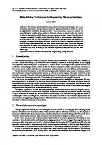
work already done before, Z IG Z AG first verifies if the extension Il+1 ∪ {y} is a retained itemset. If so, its support can be computed by just using d+ , d− , and Π, thereby enhancing the support computation process. All these procedures are described in Figure 1. Next we describe how we can parallelize the basic Z IG Z AG algorithm.

Figure 1: The Z IG Z AG Algorithm

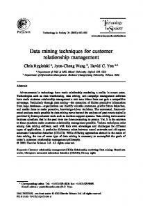
3.3 Parallel Search for Maximal Frequent Itemsets We now consider the problem of efficiently parallelizing the Z IG Z AG algorithm. The main idea of our parallel approach is to assign distinct backtrack trees to distinct processors. Figure 2 shows an illustrative example where minimum support is 30% (the framed itemsets are the maximal frequent ones, while the cut itemsets are the infrequent ones). The two different backtrack trees, each one is assigned to a different processor. Note that there is no dependence among the processors, because each backtrack tree corresponds to a disjoint set of candidates. Since each processor can proceed independently there is no synchronization while searching for maximal frequent itemsets. To achieve a suitable level of load-balancing, the backtrack trees

are assigned to the processors by using the idea of bitonic partitioning. Bitonic Partitioning (Single Backtrack Tree): In [8] a new partitioning scheme, called bitonic partitioning, for load balancing was proposed. This scheme can be applied to the problem here as well. This scheme is based on the observation that the sum of the workload due to itemsets i and (2P − i − 1) is a constant: wi + w2P−i−1 = n − i − 1 + (n − (2P − i − 1) − 1) = 2n − 2P − 1 We can therefore assign itemsets i and (2P − i − 1) as one unit with uniform work (2n − 2P − 1). If n mod 2P = 0 then perfect balancing results. The case n mod 2P 6= 0 is handled as described in [8].

Bitonic Partitioning (Multiple Backtrack Trees): Above we presented the simple case of where we only had a single backtrack tree. In general we may have multiple trees. Observe that the bitonic scheme presented above is a greedy algorithm, i.e., we sort all the w i (the work load due to itemset i), extract the itemset with maximum wi , and assign it to processor 0. Each time we extract the maximum of the remaining itemsets and assign it to the least loaded processor. This greedy strategy generalizes to the multiple backtrack trees as well, the major difference being work loads in different trees may not be distinct. Once each processor has the MFI, the supports of the subsets are counted in parallel in much the same way as the local MFI was generated. In this case, a task corresponds to finding the support count of all frequent subsets.

Figure 2: Backtrack Trees for Items A and B on ∆

3.4 Parallel and Distributed Incremental Algorithm The MFI search employed by Z IG Z AG is very efficient, but it can only be applied when the dynamic database is centralized. Now we will explain how we can extend Z IG Z AG for mining

distributed databases. We first present Lemma 1, which is the basic theoretical foundation of our approach. Lemma 1 − A global frequent itemset must be local frequent in at least one partition.

Proof. − Let C be an itemset. If C.supi < s∆ × | δi | for all i = 1, ..., n, then C.sup < s∆ × | P P ∆ | (since C.sup = ni=1 C.supi and | ∆ |= ni=1 | δi |), and C cannot be globally frequent.

Therefore, if C is a global frequent itemset, then it must be local frequent in some partition δ i .

In the first step each site Si independently performs a parallel and incremental search for MFIδi , using Z IG Z AG on its database δi . After all sites finish their searches, the result will be the set of all local MFIs, {MFIδ1 , MFIδ2 , ... , MFIδi }. This information is sufficient for

determining all local frequent itemsets, and from Lemma 1, it is also sufficient for determining all global frequent itemsets. The second step starts after all local MFIs were found. Each site

sends its local MFI to the other sites, and then they join all local MFIs. Now each site knows S the set ni=1 MFIδi , which is an upper bound for MFI∆ .

In the third step each site independently performs a top down incremental enumeration of the potentially global frequent itemsets, as follows. Each itemset present in the upper bound Sn i=1 MFIδi is broken into k subsets of size (k − 1). This process iterates generating smaller subsets and incrementally computing their support counts until there are no more subsets to be checked. At the end of this step, each site will have the same set of potentially global frequent itemsets (and the support associated with each of these itemsets). S

Lemma 2 − ni=1 MFIδi determines all global frequent itemsets. Proof. − We know from Lemma 1 that if C is a global frequent itemset, so it must be local frequent in at least one partition. If C is local frequent in some partition δl , then it must be determined by MFIδl , and S consequently by ni=1 MFIδi .

By Lemma 2 all global frequent itemsets were found, but not all itemsets generated in the third step are global frequent (some of them are just local frequent). The fourth and final step

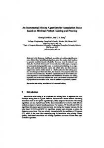
makes a reduction operation on the local support counts of each itemset, to verify which of them are globally frequent in ∆. The process starts with site S1 , which sends the support counts of its itemsets (generated in the third step) to site S2 . Site S2 sums the support count of each itemset (generated in the third step) with the value of the same itemset obtained from site S 1 , and sends the result to site S3 . This procedure continues until site Sn has the global support counts of all potentially global frequent itemsets. Then site Sn finds all itemsets that have support greater than or equal to s∆ , which constitutes the set of all global frequent itemsets, i.e., MFI∆ . We illustrate all steps of the algorithm execution in Figure 3. The transactions of ∆ (used in the example of Figure 2) were distributed in two databases δ1 and δ2 (δ1 is located in site 1, while δ2 is located in site 2). The value of the minimum support is 50%. In the first step each site mines its local MFI. The result is MFIδ1 = {ABDE, BCE}, and MFIδ2 = {ACDE, BCD}. In

the next step, all sites exchange their local MFIs, so that each one can compute the upper bound Sn i=1 MFIδi , which is {ABDE, BCE, ACDE, BCD}. Now, each site computes the support count S

of each subset of each itemset in ni=1 MFIδi . Some of the generated subsets at site Si are not local frequents in di , but their support count must be computed because some of them must be local frequent in other site, and therefore they can still be global frequent itemsets (i.e., ABE).

In the last step the global frequent itemsets are found by aggregating (sum reduction operation) the local counts of each local frequent itemset.

Figure 3: Overall Process of Distributed Mining There are two ways of doing distributed mining. The first is to do it within a cluster or a local area network. In this case, a site corresponds to a single host with its own database, which can compute the local MFI using the bag of tasks approach found in section 3.3. It can then communicate with the other hosts in the cluster or LAN according to the algorithm above to determine the global frequent itemsets. The second way of doing distributed mining is to do it across clusters. In this case, a site corresponds an entire cluster, and each cluster has its own database that is visible to all of the nodes within that cluster. Instead of assigning distinct backtrack trees to distinct processors, they are assigned to distinct nodes within the cluster. The nodes send their results to the leader node, which then generates the local MFI. The leader then communicates with the leaders of S other clusters to generate ni=1 MFIδi .

3.5 Interactive Issues 3.5.1

High-Contrast Frequent Itemsets

An important issue when mining distributed databases is to understand the differences between the databases. An effective way to understand such differences is to find the high-contrast

frequent itemsets. The support counts of such itemsets vary significantly accross different databases. We use the well-established notion of entropy to detect how the support count of a given frequent itemset is distributed accross the databases [7]. For a random variable, the entropy is a measure of the non-uniformity of its probability distribution. Let X be a global freP i quent itemset. The value pX (i) = X.sup is the probability of occurrence of X in δi . ni=1 pX (i) X.sup P

= 1, and H(X) = − ni=1 (pX (i) × log(pX (i))) is a measure of how the local support counts of X is distributed accross the different databases. Note that 0 ≤ H(X) ≤ log(n), and so

≤ 1. If E(X) is greater than or equal to a given minimum entropy 0 ≤ E(X) = log(n)−H(X) log(n) threshold, then X is classified as high-contrast frequent itemset. 3.5.2

Query Response Time

One of the goals of the distributed mining algorithm is to minimize response time to a query for the global frequent itemsets in an dynamic, distributed database. Since the database is dynamic, each site is incrementally updating its local frequent itemsets. The time it takes to update the local frequent itemsets is proportional to B =| d+ | + | d− |, that is to say, the size of a block of differences. We can view the updates to the database as a queue containing zero or more such blocks. If a query arrives while a block is being processed, there cannot be a response until the calculation of the local frequent itemsets is completed and used to find the global frequent itemsets. An obvious approach to reducing response time is to decrease the size of B. However, because of overhead, the time it takes to do two increments of size B is longer than the time it takes to do a single increment of size 2 × B. So there is a tradeoff: The larger B is, the more

up-to-date global frequent model∆ will be, since it incorporates a greater number of changes to the database, but the longer the response time to the query will be.

3.6 Discussions All extant incremental mining algorithms make use of the negative border [11] to perform the incremental operation. The basic idea is to keep the negative border up-to-date as the database is updated. As shown in [13], the size of the negative border is typically much larger than the size of MFI∆ . So updating the negative border requires many more candidates to be processed, incurring computational and I/O overhead. By updating MFI∆ , we process fewer candidates than other approaches. Almost all distributed algorithms for frequent itemset mining (CD [1], FDM [3], and DMA [6]) require a round of communication in every iteration of the algorithm. However, synchronization is implicit in communication, and therefore these algorithms suffer from excessive communication overhead. Our approach overcomes the problem of communication overhead by making use of maximal frequent itemsets. Each site can independently generate its local MFI, so no communication is needed during this search. After all local MFIs are found, only one round of communication is performed in order to build the upper bound. Again, each site

can independently enumerate the local frequent itemsets, and after all local frequent itemsets are found, only one reduction operation is needed to find the global frequent itemsets. Therefore, by making use of maximal frequent itemsets, our distributed algorithm can asynchronously mine the frequent itemsets.

4 Experimental Evaluation Our experimental evaluation was carried out on two clusters. The first cluster consists of dual P ENTIUM III 1Ghz nodes with 1GB of main memory Red Hat Linux 7.1. The second cluster consists of single P ENTIUM III 933 MHz nodes with 512 MB of memory running Red Hat Linux 7.3. We further partitioned each cluster into two virtual clusters for a total of four clusters. We assume that each database is distributed between the clusters, and that each node in the cluster has access to its cluster’s portion of the database. Within each cluster, we have implemented the parallel program using the MPI message-passing library (MPICH over GM 1 ), and for communication between clusters we use sockets. We used real and synthetic databases for testing the performance of our algorithm. The WPortal database is generated from the click-stream log of a large Brazilian web portal, and the WCup database is generated from the click-stream log of the 1998 World Cup web site, which is publicly available at ftp://researchsmp2.cc.vt.edu/pub/worldcup/. We scanned each log and produced a respective transaction file, where each transaction is a session of access to the site by a client. Each item in the transaction is a web request. Not all web requests were turned into items; to become an item, the request must have three properties: (1) the request method is GET; (2) the request status is OK; and (3) the file type is HTML. A session starts with a request that satisfies the above properties, and ends when there has been no click from the client for 30 minutes. All requests in a session must come from the same client. We also used a synthetic database (also available from IBM Almaden), which have been used as benchmarks for testing previous mining algorithms. This database mimics the transactions in a retailing environment [2]. Table 1 shows the characteristics of the real databases used in our evaluation. It shows the number of items, the average transaction length, the number of transactions, and the size of each database. Each database was partitioned into two equal halves, and each halve was placed on a separate cluster. 1

www.myricom.com

Database #Items WPortal 3,183 WCup 5,271 T5I2D8000K 2,000

Avg. Length 4 8 10

#Transactions 7,786,137 7,618,927 8,000,000

Size 428MB 645MB 1,897MB

Table 1: Database Characteristics.

4.1 Intra-Cluster Evaluation 4.1.1

Performance Comparison

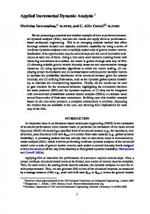
Figure 4 shows the execution times obtained for different databases, and parallel and incremental configurations. As we can see, better execution times are obtained when we combine both parallel and incremental approaches. Furthermore, when the parallel configuration is the same, the execution time is better for smaller block sizes (since the database is smaller). The improvements obtained on the real databases are not so impressive as the improvement for the synthetic one. The reason is that the real database has a skewed data distribution, and therefore the partitions of the real databases have a very different set of frequent itemsets (and therefore very different local MFIs). On the other hand, the skewness of the synthetic data is very low, therefore each partition of the synthetic database is likely to have a similar set of frequent itemsets. S

From the experiments in the synthetic database we observed that ni=1 MFIδi (i.e., the upper bound) is very similar to each local MFI. This means that the set of local frequent itemsets is very similar to the set of global frequent itemsets, and therefore few infrequent candidates are generated by each processor.

WCup - 0.5%

WPortal - 0.005%

1

2

3

4

5

6

7

100

10

8

10000

Elapsed Time (secs)

100

10

100% 20% 10% 1

2

3

# Processors WCup - 1%

4 5 # Processors

7

100

10

8

1

2

3

4

6

7

8

2

3

4 5 # Processors

7

8

6

7

8

T5I2D8000K - 1.0%

10

1

6

1000

100% 20% 10%

100

1

5

# Processors

Elapsed Time (secs)

Elapsed Time (secs)

Elapsed Time (secs)

10

3

6

1000

WPortal - 0.01%

100

2

5

1000

100% 20% 10%

1

4

100% 20% 10%

# Processors

1000

1

T5I2D8000K - 0.5%

1000

100% 20% 10% Elapsed Time (secs)

Elapsed Time (secs)

1000

6

7

8

100

10

1

100% 20% 10% 1

2

3

4 5 # Processors

Figure 4: Total Execution Times on Different Databases. 4.1.2

Improvements from Incremental Mining

We also investigated the performance of our algorithm in experiments for evaluating the speedup of different incremental configurations. In this experiment, we first mined a fixed size database, and then we performed the incremental mining for different increment sizes (5% to 20%). In order to evaluate only the incremental performance, we used the incremental algorithm with only one processor (Actually, we also varied the number of processors, but the speedup was very similar for different number of processors, so e show only the results regarding one processor). Figure 5 shows the speedup numbers of our incremental algorithm. Note that the speedup is in relation to re-mining the entire database. As is expected, the speed is inversely proportional to the size of the increment. This is because the size of the new data coming in is smaller. Also note that better speedups are achieved by greater minimum supports. We observed that, for the databases used in this experiment, the proportion of retained itemsets (itemsets that are computed by examining only d+ and Π) is larger for greater minimum supports.

WCup

WPortal

0.5% 1.0%

6

Speedup

Speedup

4 3 2

20

10

7

8

0.005% 8 0.01%

5

1

T5I2D8000K

9

18

16

14

12

10

8

6

0.5% 9 1.0%

7

6

Speedup

7

5 4

6 5 4

3

3

2

2

1

20

18

Block Size (%)

16

14

12

10

8

1

6

20

18

Block Size (%)

16

14

12

10

8

6

Block Size (%)

Figure 5: Speedups on Different Incremental Configurations.

4.2 Inter-Cluster Evaluation We also performed several sets of experiments in a broader scenario involving several clusters. The first set involved finding the number of transactions that were processed and incorporated into the global model MFI∆ when we varied certain parameters. The second set examined how the query response time was affected the block size and the query arrival time. 4.2.1

Transactions Processed WPortal - 0.01% - 1 node (2 clusters) 7e+06 6.5e+06

10% 20% 40%

4e+06

5.5e+06

# Transactions

# Transactions

6e+06

WCup - 1.0% - 1 node (2 clusters) 4.5e+06

5e+06 4.5e+06 4e+06 3.5e+06

3.5e+06 3e+06 2.5e+06 2e+06 1.5e+06

3e+06 2.5e+06

10% 20% 40%

30

35

40 45 50 Deadline (secs)

55

60

1e+06

10

15

20 25 30 Deadline (secs)

35

40

Figure 6: Number of transactions processed. The first experiment we conducted was to examine how the size of a block, the number of nodes used in each cluster, and the time at which a query arrives affects the amount of data used to build the global model MFI∆ . For the wportal database we used a minimum support of 0.01% and for the wcup database we used a minimum support of 1.0%. The results all have similar trends, and two example cases can be seen in figure 6. The X-axis represents the time elapsed from when the mining began until the query arrived (the deadline), and the Y-axis represents the number of transactions that are incorporated into the global model MFI∆ . The lines on the graph represent different values of the block size B, which is given here as percentages of the database on each cluster. The graphs show that the more time that elapses before the query arrives, the

more data that is incorporated into the model, which is to be expected. It also shows that the as the block size decreases, fewer transactions can be processed before the query arrives. This is due to the fact there is more overhead involved in processing a large number of small blocks than there is in processing a small number of large blocks.

60 50 40 30 20 10 40

45

50 55 Deadline (secs)

60

65

WPortal - 0.01% - 1 node (4 clusters) 50

10% 20% 40%

45 40 35 30 25 20 15 10 5

35

40

45

50

55

60

65

60 50 40 30 20 10

35

40

45

10% 20% 40%

80 70 60 50 40 30 20 10 10

15

20

25

30

35

40

45

50

Waiting time (secs) [avg-var, avg, avg+var]


WCup - 1.0% - 1 node (2 clusters)

5

10% 20% 40%

40 35 30 25 20 15 10

35

40

45

10% 20% 40%

40 35 30 25 20 15 10 5 10

15

20

25

30

Deadline (secs)

35

40

45

50



WCup - 1.0% - 1 node (4 clusters)

5

55

60

65

10% 20% 40%

35 30 25 20 15 10 5 0

35

40

45

10% 20% 40%

50 40 30 20 10

0

5

10

15

20

25

30

35

40

45

50

WCup - 1.0% - 2 nodes (4 clusters) 10% 20% 40%

30 25 20 15 10 5 0

5

10

15

20

25

30

Deadline (secs)

65

WPortal - 0.01% - 4 nodes (4 clusters) 10% 20% 40%

30 25 20 15 10 5

35

40

45

50

55

60

65

WCup - 1.0% - 4 nodes (2 clusters) 40

10% 20% 40%

35 30 25 20 15 10 5 0

0

5

10

15

20

25

30

35

40

45

50

45

50

Deadline (secs)

35

0

60

Deadline (secs)

WCup - 1.0% - 2 nodes (2 clusters)

0


35

Deadline (secs)

45

0

50

60

Deadline (secs)

0

65

WPortal - 0.01% - 4 nodes (2 clusters) 40

Deadline (secs)

90

0

60


Deadline (secs)

0



35

70

35

40

45

50


0

10% 20% 40%

80


10% 20% 40%

70



WPortal - 0.01% - 1 node (2 clusters) 80


Query Response Time




4.2.2


10% 20% 40%

25 20 15 10 5 0

0

5

10

15

20

25

30

Deadline (secs)

Figure 7: Query Response Time using Equal Block Sizes.

35

40

70 60 50 40 30 20 10 0

0

5

10

15

20

25

30

35

40

Deadline (secs)

45

50


3.5% - 6.5% (10% total) 7% - 13% (20% total) 14% - 26% (40% total)

45 40 35 30 25 20 15 10 5 0

0

5

10

15

20

25

30

Deadline (secs)

35

40

45

50


3.5% - 6.5% (10% total) 7% - 13% (20% total) 14%- 26% (40% total)



WCup - 1.0% - 1 node (2 clusters) 80


3.5% - 6.5% (10% total) 7% - 13% (20% total) 14% - 26% (40% total)

25 20 15 10 5 0

0

5

10

15

20

25

30

35

40

45

50

Deadline (secs)

Figure 8: Query Response Time using Different Block Sizes. In the next set of experiments we focused on the query response time, that is to say, the amount of time a user must wait before the global model is computed. For this experiment we varied the block size B (in these experiments we assume that each cluster use the same block size) and the time at which the query arrives. The results can be seen in figure 7. The X-axis again represents the time at which the query arrives, and the Y-axis represents the time spent waiting for the global model to be computed. These graphs show that as B decreases, the time to wait for a response also decreases. However, the time at which a query arrives affects the waiting time in a seemingly random manner. This is because a query arrives at some random point during the processing of a block. The time remaining to compute the local frequent itemsets is therefore a random number. The graphs above show the query response time averaged over five runs, and the vertical bars represent the variance in the runs. This set of experiments, in conjunction with the first set, clearly show the trade-off between block size and query response time: As the block size increases, the number of transactions processed also increases, but the response time increases as well. Figure 8 shows the same experiment when different block sizes across clusters are allowed. The basic idea is that smaller response times can be obtained by assigned larger blocks to the less powerfull cluster. The local model in this cluster will be updated less frequently, but in response, smaller query response times can be obtained by this approach. We can comprove this by comparing the results in Figure 8 against the respective result in Figure 7. 4.2.3

Communication

We also performed a set of experiments to analyze the communication overhead imposed by our algorithm. In particular we examined the number of bytes transferred between clusters when we varied the minimum support, the block size B, and the number of clusters involved in the computation. The results can be seen in figure 9. As is expected, as the minimum support decreases, the number of candidates will increase, and will therefore increase the number of bytes that must be transferred between the clusters, since our algorithm must exchange the support counts of every candidate processed. Also, as the block size increases, the amount of communication decreases. The reason is that for smaller block sizes the number of candidates

processed tends to be greater (assuming the same minimum support). Finally, the amount of communication required increases when more clusters are involved in the process. However, the increasing factor is not linear because the data-skewness also increases when more clusters are involved in the process, and then the number of candidates processed is increased as well. WPortal

Communication (bytes)

1.4e+06 1.2e+06 1e+06

10% (2 clusters) 20% (2 clusters) 40% (2 clusters) 10% (4 clusters) 20% (4 clusters) 40% (4 clusters)

800000 600000 400000 200000 0 0.005 0.01 0.015 0.02 0.025 0.03 0.035 0.04 0.045 0.05 0.055

WCup 6e+06

Communication (bytes)

1.6e+06

10% (2 nodes) 20% (2 nodes) 40% (2 nodes) 10% (4 nodes) 20% (4 nodes) 40% (4 nodes)

5e+06 4e+06 3e+06 2e+06 1e+06 0 0.1

0.2

0.3

Minimum Support (%)

0.4

0.5

0.6

0.7

0.8

0.9

1

Minimum Support (%)

Figure 9: Communication Overhead. 4.2.4

High-Contrast Itemsets

The last set of experiments are regarding high-contrast frequent itemsets. We utilized three databases: WPortal, WCup, and also a high-skewd synthetic database. The synthetic database was generated in the following way. We first generated four different syntethic databases: T10I2D2000K, T10I4D2000K, T10I6D2000K and T10I8D2000K. Next, each one of these databases was assigned to a different cluster. In that way, we ensure that this distributed database contains high-skewed data. We varied three parameters: the minimum support, the number of clusters involved in the process, and the minimum entropy. Figure 10 shows the results obtained in each database. As we can observe, very different results were obtained from each database. The percentage of high-contrast frequent itemsets is interesting here because it to some extents reveals the skewness of the database. From the experimental result, we know that WCup database is more skewed than WPortal dataibase, considering given the same support thresholds for these two databases, WCup will give a much higher percentage of high-contrast frequent itemsets. Usually the percentage of high-contrast frequent itemsets will be decremented when minimum support threshold going up. This is quite understandable considering when the support threshold is low, there will be a large number of global frequent itemsets generated, and quite a lot itemsets amongest these itemsets become global frequent only because they are frequent highly enough local in some site. By contrast, when the support threshold getting higher, it’s getting harder for a local frequent itemset to become global frequent, which means a loss of high-contrast frequent itemsets. Accordingly there is a higher proportion of high-contrast frequent itemsets in the former scenario. Meanwhile, the more clusters on which the data distributed, the greater possiblily of the skewness of the data. This is verified by the experimental data. It’s interesting to notice

that for the high-skewed synthetic data, when the support threshold incremented from 0.05 to 0.1, the percentage of high-contrast frequent itemsets did not increase as expected. We guess this can be attributed to the high skewness of the data. We surmise for such data there exists some threshold for our claim to take effect. Take our synthetic data as an example, the threshold value is around 0.1. Before this threshold, when we raised the support value, both of the high-contrast frequent itemsets and the global frequent itemsets became less, but the loss of the former was dominated by the latter, eventually leading to a raised percentage of high-contrast frequent itemsets.

45 40

0.1 (2 clusters) 0.02 (2 clusters) 0.1 (4 clusters) 0.02 (4 clusters)

35 30 25 20 15 10 5 0 0.005 0.01 0.015 0.02 0.025 0.03 0.035 0.04 0.045 0.05 0.055 Minimum Support (%)

90 80 70

High-Skewed Synthetic Data Percentage of High-Contrast Itemsets

50

WCup Percentage of High-Contrast Itemsets

Percentage of High-Contrast Itemsets

WPortal 55


60 50 40 30 20 10 0 0.1

0.2

0.3

0.4

0.5

0.6

0.7

0.8

0.9

1

90 80 70 60 50 40 30 20 10


0 0.05 0.1 0.15 0.2 0.25 0.3 0.35 0.4 0.45 0.5

Minimum Support (%)

Minimum Support (%)

Figure 10: High-Contrast Frequent Itemsets.

5 Conclusions In this paper we considered the problem of mining frequent itemsets on dynamic, distributed databases in different parallel and distributed environments. We presented an efficient distributed and parallel incremental algorithm to deal with this problem. In particular we present techniques to minimize the response time to a query for the global set of frequent itemsets, as well as to find high-contrast frequent itemsets. Our experiments examined the trade-offs involved in minimizing the query response time (whether to sacrifice query response time in order to incorporate more transactions in the model), the amount of data transferred between clusters, and how the distribution of the data affected the number of high-contrast frequent itemsets. Our future work involves using sampling techniques to minimize the query response time and how to minimize query response time in wide-area networks, were communication latencies tend to be relatively large.

References [1] R. Agrawal and J. Shafer. Parallel mining of association rules. In IEEE Trans. on Knowledge and Data Engg., volume 8, pages 962–969, 1996.

[2] R. Agrawal and R. Srikant. Fast algorithms for mining association rules. In Proc. of the 20th Int’l Conf. on Very Large Databases, SanTiago, Chile, June 1994. [3] D. Cheung, J. Han, V. Ng, A. Fu, , and Y. Fu. A fast distributed algorithm for mining association rules. In 4th Intl. Conf. Parallel and Distributed Info. Systems, 1996a. [4] D. Cheung, J. Han, V. Ng, and C. Y. Wong. Maintenance of discovered association rules in large databases: An incremental updating technique. In Proc. of the 12th Int’l. Conf. on Data Engineering, February 1996. [5] D. Cheung, S. Lee, and B. Kao. A general incremental technique for maintaining discovered association rules. In Proc. of the 5th Int’l. Conf. on Database Systems for Advanced Applications, pages 1–4, April 1997. [6] D. Cheung, V. Ng, A. Fu, , and Y. Fu. Efficient mining of association rules in distributed databases. In IEEE Trans. on Knowledge and Data Engg., volume 8, pages 911–922, 1996. [7] D. Cheung and Y. Xiao. Effect of data skewness in parallel mining of association rules. In Proc. of the 4th Pacific-Asia Conference on Knowledge Discovery and Data Mining, pages 48–60, New York, USA, August 1998. [8] M. Cierniak, M. Zaki, and Wei Li. Compile-time scheduling algorithms for a heterogeneous network of workstations. In The Computer Journal, volume 40, pages 356–372. [9] V. Ganti, J. Gehrke, and R. Ramakrishnan. Demon: Mining and monitoring evolving data. In Proc. of the 16th Int’l Conf. on Data Engineering, pages 439–448, San Diego, USA, 2000. [10] K. Gouda and M. Zaki. Efficiently mining maximal frequent itemsets. In Proc. of the 1 st IEEE Int’l Conference on Data Mining, San Jose, USA, November 2001. [11] S. Lee and D. Cheung. Maintenance of discovered association rules: When to update? In Research Issues on Data Mining and Knowledge Discovery, 1997. [12] S. Thomas, S. Bodagala, K. Alsabti, and S. Ranka. An efficient algorithm for the incremental updation of association rules. In Proc. of the 3rd ACM SIGKDD Int’l Conf. on Knowledge Discovery and Data Mining, August 1997. [13] A. Veloso, W. Meira Jr., M. B. de Carvalho, B. Poˆ ssas, S. Parthasarathy, and M. Zaki. Mining frequent itemsets in evolving databases. In Proc. of the 2nd SIAM Int’l Conf. on Data Mining, Arlington, USA, May 2002.

[14] A. Veloso, W. Meira Jr., M. B. de Carvalho, B. Rocha, S. Parthasarathy, and M. Zaki. Efficiently mining approximate models of associations in evolving databases. In Proc. of the 6th Int’l Conf. on Principles and Practices of Data Mining and Knowledge Discovery in Databases, Helsinki, Finland, August 2002. [15] M. Zaki, S. Parthasarathy, M. Ogihara, and W. Li. New parallel algorithms for fast discovery of association rules. Data Mining and Knowledge Discovery: An International Journal, 4(1):343–373, December 1997.