arXiv:quant-ph/0401075v2 26 Jul 2004. Simulating Causal ... 2A9, Canada. b Department of Physics, Queen Mary, University of London, London E1 4NS, UK.
Simulating Causal Wave Function Collapse Models
arXiv:quant-ph/0401075v2 26 Jul 2004
Fay Dowkera and Isabelle Herbautsb
Abstract We present simulations of causal dynamical wave function collapse models of field theories on a 1 + 1 null lattice. We use our simulations to compare and contrast two possible interpretations of the models, one in which the field values are real and the other in which the state vector is real. We suggest that a procedure of coarse graining and renormalising the fundamental field can overcome its noisiness and argue that this coarse grained renormalised field will show interesting structure if the state vector does on the coarse grained scale. We speculate on the implications for quantum gravity.
a
Blackett Laboratory, Imperial College, London SW7 2BZ, UK and Perimeter Institute, Waterloo, Ontario N2T
2A9, Canada. b
Department of Physics, Queen Mary, University of London, London E1 4NS, UK.
1
Introduction
The tension between relativity and quantum theory exists even before one tries to include gravity in the picture and even if one tries to take a determinedly operationalist stance one is forced to try to make a careful statement of what quantities may be measured and how (e.g. [1, 2]). If one is seeking an observer independent alternative to standard quantum theory, however, then that tension escalates into an issue of fundamental importance, whose resolution may lead to the “radical conceptual renewal” anticipated by John Bell [3]. This conceptual advance may be intimately linked with progress in finding a quantum theory of gravity, for example by finding the correct, quantum analogue of the “Bell Causality” condition for causal sets [4] but we have a more modest objective in this paper. We will investigate a simple observer independent dynamical collapse model on a lattice which is causal in the sense that external agents cannot manipulate it to communicate faster than the lattice causal structure ought to allow [5]. The model in question is a model for a discrete quantum field theory and it falls in the general category of “dynamical localisation” models (for a substantial review see [6]). It can be thought of as a causal, discrete Continuous Spontaneous Localisation (CSL) model [7, 8, 9]. Dynamical collapse models admit (at least) two possible interpretations. In the first, which we call the State Interpretation (SI) and which is used by almost all workers in this area, it is the state vector which is real (see for example [10]). In the second, which we call the Field Interpretation (FI), it is the field values which are real (in the original GRW model [11] the analogous interpretation first proposed by Bell [12] and championed by Kent [13, 14] is that the collapse centres are real). This choice of interpretation is not something that is often highlighted. We believe that it is a physical choice and it is one of the purposes of the current paper to investigate the consequences of the choice. It may be that SI and FI are operationally indistinguishable in which case there is less motivation for considering one over the other, though each may suggest different directions for future research. It may be that the interpretations lead to verifiably different predictions which would be an extremely interesting result. So far, almost all work on collapse models and comparisons of their implications with experiment have assumed the SI. We would like to take a small step towards determining whether the FI has anything interesting to say about the real world by investigating it in the context of our lattice model. The paper is structured as follows. In section 2 we review the lattice collapse models of [5]. In section 3 we describe our simulations of the SI and the FI, for a range of parameters for some simple initial states. In section 4 we investigate the decay of superpositions. Section 5 is a description of coarse graining and renormalisation in the model. Section 6 contains a discussion of parameters, a description of future work and speculations on applications to quantum gravity.
1
2
1+1 lattice collapse models
In order to motivate the lattice collapse models, we first review the GRW model, following the presentation of Kent [14] who calls it the “ur-model” of modern dynamical collapse models. In the GRW model for a single spinless particle in one dimension the wave function ψ(x, t) undergoes two types of evolution. Almost all of the time, it follows the Schr¨odinger equation, but at discrete randomly chosen times it jumps discontinuously, so that ψ→ R
where Jxˆ is the function of x
1
Jxˆ ψ dx|Jxˆ ψ|2 1
� 21 ,
Jxˆ (x) = a− 2 π − 4 e−(x−ˆx)
2
/2a2
(2.1)
.
The x ˆ is chosen randomly according to the probability distribution Z Prob(ˆ x) = dx|Jxˆ ψ|2 which is properly normalised to be a probability distribution because Z dˆ xJxˆ (x)2 = 1 .
(2.2)
(2.3)
(2.4)
a is a constant parametrising the model. The times of the jumps are given by a Poisson process, with mean interval τ /N between jumps. The parameters τ and a are to be thought of as new constants of nature; GRW originally suggested τ ≈ 1015 sec.
a ≈ 10−5 cm,
(2.5)
In the interpretation of the GRW model due to Bell, it is the sequence of stochastically generated events – (ˆ x, t)’s – which constitutes reality in the model and the model assigns a probability distribution to the sample space of all such sequences, (ˆ x1 , t1 ), . . . (ˆ xn , tn ), which is the probability of that sequence of times (Poisson distributed) multiplied by kJxˆn U (tn , tn−1 ) . . . Jxˆ1 U (t1 , t0 )ψ(t0 )k2
(2.6)
where U (ti+1 , ti ) is the standard Schr¨odinger time evolution operator between two collapse times. The lattice collapse models aim to emulate the formalism of the GRW model in the context of a field theory with non-trivial causal structure. They are based on light cone lattice field theories in 1+1 dimensions, introduced in the study of integrable models [15]. We follow the presentation of Samols [16] of this “bare bones” local quantum field theory. Spacetime is a 1 + 1 null lattice, periodically identified in space with N spatial vertex sites. The links of the lattice are left or right going null rays. A spacelike surface, σ, is given by the set of links cut by the surface and is specified completely by the position of an initial link and a sequence of N right-going and N left-going links, moving from left to right, starting with the initial link. An example is shown in figure 1.
2
σ/
1
/
2
/
σ
v 1
2
σt
Figure 1: The light-cone lattice. σt is a constant time slice; σ is a general spacelike surface and σ ′ one obtained from it by an elementary motion across the vertex v. Links labelled 1 and 2 (1′ and 2′ ) are the ingoing (outgoing) links at v. The local field variables, α, live on the links. At link l the variable αl takes just two values, 0 or 1, and there is a (“qubit”) Hilbert space, Hl , spanned by two states labelled by αl = 0 and αl = 1. At each vertex, v, the local evolution law is given by a 4-dimensional unitary R-matrix, U (v), that evolves from the 4-d Hilbert space that is the tensor product of the Hilbert spaces on the two ingoing links to the 4-d Hilbert space on the two outgoing links. A quantum state |Ψσ i on a spacelike surface, σ, is an element of the 22N -dimensional Hilbert space, Hσ , that is the tensor product of the Hilbert spaces on all the links cut by σ. The α basis vectors of Hσ (the only ones we will use: they form the preferred or physical basis) are labelled by the possible field configurations on σ, namely the 2N -element bit strings {0, 1}2N . We identify the Hilbert spaces
on different surfaces in the obvious way by identifying 2-dimensional Hilbert spaces on links vertically above and below each other on the lattice. In the standard quantum theory, the unitary evolution of the state to another spacelike surface σ ′ is effected by applying all the R-matrices at the vertices between σ and σ ′ , in an order respecting the causal order of the vertices. In the simplest case, when only a single vertex is crossed (to the future of σ) the deformation of σ to σ ′ is called an “elementary motion” and an example is shown in figure 1. The R-matrices are left unspecified for now to keep the discussion as general as possible. In a conventional field theory, they will be uniform over the lattice. We assume that there is an initial spacelike surface, σ0 , with a state, |Ψ0 i, on that surface. We consider the lattice to extend into the infinite future. The lattice vertices to the future of σ0 are partially ordered by their spacetime causal order. We define a stem to be a finite subset of the vertices to the future of σ0 which contains its own past (to the future of σ0 ). Consider a natural labelling of all the vertices to the future of σ0 : v1 , v2 , v3 . . . so that if vi is in the causal past of vj then i < j. This is a linear extension of the partial order and the finite set {v1 , v2 . . . vk } is a stem for any k. We also introduce the notation σk to denote the spacelike surface reached after the elementary motions across v1 , v2 . . . vk have been completed. There is a one-to-one correspondence between stems and spacelike surfaces to the future of σ0 .
3
On each link (ı.e. on each 2-dimensional Hilbert space associated with a link) we consider the two jump operators J0 and J1 where 1 J0 = √ 1 + X2
� 1 0
0 X
�
1 J1 = √ 1 + X2
,
� X 0
0 1
�
,
(2.7)
and 0 ≤ X ≤ 1. These would be projectors onto states |0i and |1i respectively if X = 0. They satisfy J02 + J12 = 1 and are known as “Kraus” operators.
It is convenient to introduce the notation α ˆ vk to denote the values of the α field variables on the two outgoing links (one left and one right) from the vertex vk . Then the possible values of α ˆ vk are {(0, 0), (0, 1), (1, 0), (1, 1)} and we define the jump operator J(ˆ αvk ) on the 4-dimensional Hilbert space on the outgoing links from vk as the tensor product of the two relevant 2-dimensional jump operators, e.g. when α ˆ vk = (0, 0), J(ˆ αvk ) = J0 ⊗ J0 . We promote J(ˆ αvk ) to an operator on the Hilbert space of any spatial surface containing those two links by taking the tensor product with the identity operators on all the other components of the full Hilbert space and, finally, we define a “Heisenberg picture” operator Jvk (ˆ αvk ) ≡ U −1 (v1 ) . . . U −1 (vk )J(ˆ αvk )U (vk ) . . . U (v1 ) .
(2.8)
ˆ vn } is given by The probability of the field configuration {α ˆ v1 , . . . α αv1 )|Ψ0 ik2 . αvn ) . . . Jv1 (ˆ ˆ vn ) = kJvn (ˆ P (ˆ αv1 , . . . α
(2.9)
This depends only on the (partial) causal order of the vertices because any other choice of natural labelling of the same vertices gives the same result (because the operators at spacelike vertices commute). It is only the limitation of our mathematical notation that means we have to specify a linear extension to write down the formula (2.9). These probabilities of the field configurations on all the stems are enough, via the standard methods of measure theory, to define a unique probability measure on the sample space of all field configurations on the semi-infinite lattice. The probability (2.9) can also be written in terms of the “Schr¨odinger Picture” operators J(ˆ αvk ) αv1 )U (v1 )|Ψ0 ik2 . αvn )U (vn ) . . . J(ˆ ˆ vn ) = kJ(ˆ P (ˆ αv1 , . . . α
(2.10)
The state on the surface σn that is reached after the elementary motions over vertices v1 , . . . vn and the ˆ vn } have been realised is the normalised state field values {α ˆ v1 , . . . α |Ψn i =
αv1 )|Ψ0 i J(ˆ αvn ) . . . J(ˆ αv1 )|Ψ0 ik kJ(ˆ αvn ) . . . J(ˆ
(2.11)
where this is given in terms of the Schr¨odinger operators, J(ˆ αvk ). Note that, given a particular realised field configuration on the whole lattice, the state on any arbitrary spacelike surface can be calculated and it is independent of the linear ordering of the vertices to its past that is chosen in order to write it down. The Field Interpretation FI is captured by the slogan, “the field values are real”. Reality is rooted in spacetime. This is a covariant interpretation because nothing depends on the linear order chosen to
4
express the probability: the joint probability distribution on the field values on the lattice depends only on the causal order of the vertices. Any total ordering used in the analysis is entirely fictitious and unphysical. One can maintain a “block universe” perspective in which the reality is the whole semiinfinite lattice to the future of σ0 with a field configuration on it. It is also possible, however, to have a more “dynamic” picture of the model in which the “events” (realisations of field values on the outgoing links of a vertex) occur but with the order in which they occur physically being a partial order. The essence of the State Interpretation SI is, “the state is real”. The fundamental arena of reality is Hilbert space. Given a particular realisation of the field on the entire lattice, there is a unique state associated with each spacelike surface. The SI is covariant in the sense that the state on a spacelike surface is independent of the linear order of the vertices to its past chosen to write down the state mathematically (as in (2.11)). However, as we will see, defining local quantities on the lattice – which is necessary in order to make predictions – will bring in a dependence on hypersurfaces. We have described two possible interpretations of the formalism, SI and FI. There is another, suggested by Lajos Di´ osi and Gerard Milburn [17], which is that it describes, in the standard (no-collapse) quantum theory, an open system coupled to local ancilla systems on each link which are themselves measured. The field values then label the particular outcomes of these ancillae measurements. Alternatively, if the ancilla states are traced over, this would give rise to a density matrix, identical to that obtained by summing |ΨihΨ| (where |Ψi is given by (2.11)) over the field configurations weighted by their probabilities. The individual histories we consider in FI and SI would then be thought of as a particular “unravelling” of the evolution of this reduced density matrix. Since the lattice field theories (without collapse) described here have been interpreted as “quantum lattice gas automata” (QLGA) [18] we could therefore interpret the present work as investigations into the effects of environmental decoherence on these interesting proposed architectures for quantum computation.
3
Comparing the SI and FI for various parameters
The field variables on the lattice links take only two values, αl = {0, 1}. These values can be thought of as occupation numbers, so that an “occupied” |1i or “empty” |0i state can be associated to each link. The diagonal links of the lattice are the possible world-lines for propagation forwards in time of “bare” particles, moving either right or left and the lattice consists therefore of an array of nodes that can be occupied by left or right moving particles. These bare particles would not however, become the physical particles in a eventual continuum theory [15]. The local evolution law at each vertex on the lattice is encoded in a 4-dimensional unitary R-matrix, whose entries are the amplitudes connecting the four possible states on the ingoing and outgoing pairs of links at that vertex. Different conservation laws can be imposed on the dynamics of a system by a suitable choice of the R-matrix, describing the different processes that can take place on the lattice. For a field theory with spacetime translation invariance, the R-matrices are also chosen to be uniform
5
over the lattice. One special choice is a particle number preserving matrix, i.e. a R-matrix conserving occupation numbers at each vertex. Such a matrix can be parametrised as: տ
1 ր 0 U= 0 տ տր 0
ր
0 ie
iα
0
sin θ
e
iα
cos θ
eiα cos θ
ieiα sin θ
0
0
րտ
0 0 . 0 eiβ
(3.1)
The local unitary evolution given by the R-matrix (3.1) imposes both particle number conservation and parity invariance (symmetry under left-right exchange) throughout the lattice. An R-matrix of this type leads to a particular fermionic model, the massive Thirring model, in a suitable continuum limit of the unitary (no collapse) theory [15]. Each of the six non-zero amplitudes can be thought of as indicating possible paths for a particle at each vertex. These paths are symbolically indicated in equation (3.1) by տ for a left moving particle, ր for a right moving particle. Without loss of generality, the “nothing to nothing” amplitude is chosen to be 1. The “interaction” term between two ingoing particles is a phase multiplication only, eiβ . For the simulations presented in this paper, we set α and β to 0. Variation of θ controls the average speed of the particles on the lattice: if θ = π/2 the R-matrix is proportional to the identity matrix, and the particles change direction at each vertex and there is no propagation in space and the particles have infinite “mass”. At the other extreme, with θ = 0 the R-matrix interchanges the states on the two incoming links, so that the particles never change direction and follow null lines on the lattice and can be thought of as massless. In our simulations we are limited as to lattice size by the exponential growth of the problem in vertex number. For a lattice with N vertices, this means handling vectors with 22N components, and dealing with N multiplications of these vectors by matrices of dimensions 22N × 22N at each time step (each constant time slice). We ran simulations for N = 8, 9 and 10. The simulation proceeds in stages as follows. Given the evolution up to surface σn (in other words we have the surface, realised field values at all vertices between σ0 and σn and the normalised state on σn , |Ψn i, depending on those past realised values according to (2.11)), an elementary motion is chosen at random from those possible with equal probability. The motion is implemented resulting in a new hypersurface σn+1 and and the state is unitarily evolved to a state on σn+1 ˜ n+1 i = U (vn+1 )|Ψn i . |Ψ
(3.2)
Field values at the new vertex vn+1 (strictly, on the two outgoing links from the new vertex) are chosen at random according to the probability distribution ˜ n+1 ik2 . Prob(ˆ αn+1 ) = kJ(ˆ αn+1 )|Ψ
6
(3.3)
This is the conditional probability distribution on field values at vn+1 given the field values that have already been realised to the past of σn . If the field value α ˆ n+1 is realised then the state is “hit” and becomes the new state on σn+1 |Ψn+1 i =
˜ n+1 i J(ˆ αn+1 )|Ψ ˜ kJ(ˆ αn+1 )|Ψn+1 ik2
(3.4)
and the process repeats. Note that this evolution scheme is tantamount to putting a specific probability distribution on linear orderings of the vertices – fixed by the rule for choosing elementary motions at random with equal probability from those possible at each stage – and choosing one particular linear ordering according to that probability distribution. The distribution we have chosen is generated by a Markovian rule for evolution and thus is particularly easy to simulate. Other rules can be chosen – for example, one might choose to weight all linear orderings equally. Due to the fact that the probability distribution on the field configurations depends only on the causal order of the vertices, the results of the simulation for the field values do not depend on the choice of distribution for the linear order: any choice will lead to a correct simulation of the physical distribution on field configurations (we could even choose a fixed linear ordering with, for example, increasing labels from left to right, row by row). In the simulation of the evolution of the state, however, the probability distribution on linear orderings does play a role because a linear ordering is equivalent to a sequence of surfaces and in the simulation, the state is only calculated on the surfaces that are included in the chosen sequence. Even so, the state can still be thought of as covariant because it is determined on every surface by the realised field configuration, even though our simulation doesn’t actually calculate it. We will show two types of plots. In both of them each cell corresponds to a single link of the lattice (so that there are two cells per vertex), as shown in figure 2.
Figure 2: The cells on the light-cone lattice. The lattice is represented by an array of square cells, each cell containing one link on a diagonal. One such cell is shown by the shaded area. In one type of plot (FI) the cell is white if the field value is 0 and black if the field value is 1. In the second type (SI) the darkness of the cell is (positively) proportional to the square of the amplitude (according to the state at that stage of the evolution) for the field value 1 on the link. (in other words
7
the plot is of “stuff” [10]). It is important to emphasize that this SI plot is not the probability that the field value on the link will be 1. Indeed, let the link in question be l and suppose, at some stage in the dynamics, l is one of the outgoing links from the vertex that has just been evolved over. Let the state on the current spacelike surface through l be denoted schematically by |Ψi = a|0i + b|1i
(3.5)
where |0i (|1i) is short hand for the normalised superposition of all the terms in the state in which the value of the field on l is 0 (1). The probability that the field will be 1 on l (conditional on the past evolution to that stage) is
|a|2 X 2 + |b|2 , 1 + X2
(3.6)
whereas the square of the amplitude for field value 1, which we show in the SI plot, is |b|2 . Here, in defining this local quantity on the lattice that we can plot and analyse, we have introduced a dependence on spacelike surfaces (and hence on the choice we have made of a probability distribution on sequences of surfaces). Since, although the state on a surface is a covariant quantity, the value of |b|2 on a link is not covariant because it depends on the state on an entire surface through that link:
choose a different surface and the value of |b|2 will be different (due to the non-unitarity of the hits). In our simulation, the surface through the link is whatever it happens to be at that stage of the evolution – in other words the surface is chosen at random according to the probability distribution on surfaces defined by the Markovian evolution rule for elementary motions. So our state plot of the quantity |b|2 depends on that choice. A different choice (e.g. equally weighted linear orderings of vertices, or one fixed deterministic ordering) would give a different state plot. Alternatively, a covariant choice for the surface to use in calculating |b|2 on a link – not equivalent to any kind of “evolution” law for surfaces, stochastic or otherwise – would be the boundary of the causal past of the vertex from which the link is outgoing. We have not investigated these alternatives. In figure 3 the plots are grouped in pairs (a,b), (c,d) and (e,f) of (SI, FI) plots. The members of a pair have the same parameters and the plots in the pair refer to exactly the same run. The initial state is a field eigenstate with two particles and θ = π/6 in all three pairs. The pairs have different values of X: X = 0.1 for (a,b), 0.3 for (c,d) and 0.95 for (e,f). The plots all begin on the row of links immediately above the initial surface because there are no field values on the initial surface itself. We can see that when the jump operators are close to being projectors the state remains very close to being in an eigenstate: the R-matrices introduce superpositions which are essentially killed at each step by the jump operators. The two plots (a) and (b) in figure 3 are virtually identical, as they should be and the trajectories seen are very close to being classical random walks. Indeed, if X were exactly 0, they would be classical (non-Markovian) random walks where, at each vertex, the walker either continues in the null direction it is going in with probability cos2 (π/6) = 3/4 or changes direction with probability sin2 (π/6) = 1/4.
8
As X is increased with fixed θ, the balance changes and more signs of superposition appear in the SI plot whilst the field plot starts to look much more noisy. For X = 0.95, the state plot resembles the unitary dynamics shown in the right hand plot of figure 9 in [18] and the field plot has no discernable structure any more. The same trend is apparent in figure 4 which shows three runs with initial state a field eigenstate with 4 particles and with θ = 4π/9. The plots are again grouped in (SI, FI) pairs (a,b), (c,d) and (e,f) with three different choices of X, X = 0.1, 0.5 and 0.93 respectively. The particles trajectories are close to being vertical because θ is close to π/2 illustrating how θ controls the speed of the particles on the lattice.
Figure 3: Pairs (a,b), (c,d) and (e,f), of (SI, FI) plots for three different runs of the simulation. The initial state is a field eigenstate with two particles and θ = π/6 in all three pairs. The pairs have different values of X: X = 0.1 for (a,b), 0.3 for (c,d) and 0.95 for (e,f).
9
Figure 4: Pairs (a,b), (c,d) and (e,f), of (SI, FI) plots for three different runs of the simulation. The initial state is a field eigenstate with four particles and θ = 4π/9 in all three pairs. The pairs have different values of X: X = 0.1 for (a,b), 0.5 for (c,d) and 0.93 for (e,f).
4
Collapse of superpositions
In order to fully justify the title “dynamical collapse model” it needs to be shown that when only small numbers of degrees of freedom are involved, the model behaves virtually indistinguishably from ordinary quantum mechanics but that superpositions of “macroscopically different” states collapse rapidly. We will present analytic and numerical evidence that this is so – to the extent that we can interpret “macroscopic” – if we tune the parameter X to be sufficiently close to 1. We can see that as X gets close to 1, the realised field configurations become more and more noisy until it is impossible to discern any structure by eye (as seen for example in figure 3 (f)). Indeed when X = 1, the behaviour of the field is just that of independent choices of 0 or 1 on each link with probabilities 1/2 and 1/2. The state, on the other hand, decouples from the field and evolves deterministically according to the standard unitary evolution. It seems likely that tuning X to be close to 1 will allow us to make
10
the dynamics of the state as close as we like to ordinary Schr¨odinger evolution for as long as we choose. Since we are aiming to make a comparison to ordinary quantum mechanics we study only the SI in this section. Let X = 1 − ǫ with 0 < ǫ 0 and the vacuum state |00 . . . 0i, with particle number preserving R-matrix, the state is
preserved and the stochastic field dynamics is an independent choice on each link of 0 with probability 1/(1+X 2 ) and 1 with probability X 2 /(1+X 2 ). For the coarse grained field we again have the statistics of a binomial distribution with mean µ = X 2 /(1 + X 2 ) = 1/2 + O(ǫ) and variance σ 2 = X 2 /(2(1 + X 2 )2 M ). Let us call this the vacuum distribution for a particular ǫ. We want to “subtract” this fluctuating vacuum background and see if the remaining field has interesting features. The difference, for each block, between the mean of the vacuum distribution on coarse grained field values and the mean of the distribution corresponding to a general initial state will be of order ǫ and so to “see” these differences we need to renormalise the field. Given a block size m we define a renormalised field in the following way. Let αm be the average value of the field in an m × m block. Then the renormalised field in that block is −1 αR (αm − X 2 /(1 + X 2 )) . m = ǫ
(5.1)
Although the underlying (bare) field values are only 0’s and 1’s and the averaged field values therefore lie between 0 and 1, the renormalised values extend over a larger and larger range as m increases (with large field values exponentially unlikely). We want this renormalised field not to be swamped by vacuum fluctuations and so we need the square root of the variance of the distribution to be much smaller than the difference in the means, which implies that mǫ ≫ 1. Note that if a continuum limit were taken with a the lattice spacing going to zero, it would be reasonable for ma – the physical “discrimination scale” – to remain fixed. In which case m = O(a−1 ) = O(ǫ−2 ). We see that is hard to simulate this coarse grained field dynamics for small ǫ because our lattice size doesn’t allow the large block size that would be needed. Instead we offer the following argument as to why it is plausible that the theory is non-trivial. As a substitute for showing the field values themselves, we consider renormalised and enhanced
15
probabilities on the links. Consider, at some stage in the dynamics, the link l which is one of the outgoing links from the vertex that has just been evolved over. Then the state on the surface through l is given by (3.5) and the probability that the field will be 1 on l is given by (3.6). When ǫ is very small, this probability is within order ǫ of the vacuum value X 2 /(1 + X 2 ). Subtracting off this vacuum probability, and enhancing the contrast by dividing this by ǫ, we obtain the value |b|2 (to order ǫ). This is exactly the quantity we show in the SI plots (it is the stuff). We are led to the conclusion that when the state shows structure on some coarse grained scale, it is likely that the renormalised coarse grained field also will and we find a strong connection between the Field and State Interpretations.
6
Discussion
We have presented analysis and numerical simulations of lattice models that can be thought of as dynamical collapse models on a discrete spacetime with a fixed causal structure. At the very least the discreteness and finiteness of the model allows us to see clearly the elegant mechanism of the dynamical localisation models of Ghirardi, Rimini, Weber and Pearle at work. The competition between collapse fuelled by the stochasticity and the Hamiltonian evolution is seen clearly: the jump operators suppress superpositions in the field eigenstates and the R-matrices reintroduce them at each step. We have highlighted the choice between the State Interpretation and the Field Interpretation. We have emphasised the fact that the SI struggles to be covariant in the presence of a non-trivial causal structure due to the dependence of local quantities on a choice of hypersurface through the local region on which the quantity is defined. The FI on the other hand is manifestly covariant and respects the causal structure. We have presented evidence that the Field Interpretation can remain interesting, through the noise, by coarse graining and renormalising the fundamental field configurations. This clearly has some attractive features: there really are vacuum fluctuations at some fundamental scale but coarse graining washes them out. It remains to be discovered whether, for a value of ǫ close enough to zero to maintain microscopic superpositions, the renormalised coarse grained field has interesting structure. The fact that the linear size of the coarse graining blocks must grow as ǫ gets small means that we cannot look for this directly in our simulations on small lattices. However, we have shown that this question is closely related to the behaviour of the state on coarse grained scales: if the SI predicts interesting coarse grained structure then so does the FI. An interesting issue that arises for collapse models especially in the relativistic context, is that of energy conservation. The consensus seems to be that collapse models – and non-unitary evolution in general – if local and causal will tend to violate energy-momentum conservation, more or less severely. In the GRW model, that can be seen simply by noting that the collapses tend to cause wavepackets to narrow in position and so to broaden in momentum. These conclusions, however, have been drawn in
16
the SI in which the state is used to calculate the various quantities. The question of whether energymomentum conservation holds, and if not how large the violations will be, will have to be readdessed in the FI where it is likely to take on rather a different character. For example, the fundamental field configurations fluctuate wildly (in the continuum, they would be non-differentiable and perhaps not even continuous) and so a microscopic definition of energy, say, would not be possible. A definition depending on some coarse graining would be necessary. We leave these questions open for now. The FI suffers from the defect that it is necessary to know the state on a spacelike surface in order to predict the future behaviour of the field. It seems strange therefore not to ascribe reality to the state as well. Indeed, the interpretation in which both the stochastic quantity (here the field) and the state vector are real has been proposed by Di´ osi in many works over the years (already implicitly in [7]). There is no getting around the reality of the state if one wants to maintain a Markovian dynamics, but if one is prepared to give up the Markovian condition, it might be possible to show that the state on a spatial surface is actually determined, for all practical purposes, by the realised field values that have occured in the past back to some time depth Tmemory . We will report on work bearing on this issue in a future paper. In the original GRW model there are two parameters, essentially the microscopic decay time, Tdecay , for collapse of a superposition of a single particle in two different positions and the spatial “discrimination” scale, Xdiscrim , which is the smallest distance that the collapse can resolve. In the GRW model the values Tdecay = 1016 s and Xdiscrim = 10−5 cm are chosen. These two parameters appear in the current setting incarnated as the lattice spacing and the parameter ǫ. Given a fixed lattice spacing, demanding a particular value for Tdecay fixes the discrimination scale in the following way. Let T0 be the lattice spacing in time so that X0 = cT0 is the lattice spacing in space. Since the decay time scales like ǫ−2 we have that Tdecay = kT0 ǫ−2 where k is a dimensionless number that depends on the dynamics i.e on the R-matrix. The discrimination length scale is Xdiscrim = mX0 where m is the number of vertices in one coarse graining block dimension. We know that K ≡ mǫ ≫ 1. Putting these together we obtain Xdiscrim
1
= Kk − 2 X0 1
�
Tdecay T0
� 12
= Kk − 2 × 10⁻³ cm
(6.1) (6.2)
if we choose Tdecay ∼ 1016 s as in the GRW and CSL models and make a “natural” choice for the lattice spacing, namely the Planck scale (X0 = 10−33 cm). Xdiscrim is in danger of being too large, because K ≫ 1. But if the R-matrix can be tuned to compete with the collapse mechanism to the extent that √ k is large enough so that K/ k ∼ 10−2 then we can obtain the GRW value. There is therefore a hint that one of the extra physical constants of the GRW/CSL models can be eliminated by invoking a fundamental spacetime discreteness at the Planck scale. This is to be regarded as merely a hint for several reasons including the fact that the diamond
17
lattice used here is not Lorentz invariant. In order to produce a model that has a chance of being Lorentz invariant we would either have to take the continuum limit of the lattice models (and deal with the issues that arise there: non-physicality of the “bare” particles, the fact that the physical vacuum contains infinite numbers of bare particles etc.) or build a collapse model on a Lorentz invariant discrete structure to which Minkowski spacetime is an approximation. The only known example of the latter is a causal set, which can be thought of as a discrete “random sampling” of the causal structure of Minkowski spacetime [20, 21]. While it seems possible formally to write down a collapse model on a general causal set, with Hilbert spaces on the links and “local” evolution and collapse rules, the analysis and simulation of such a model is immensely more challenging. General models of this type have been considered [22] in which the jumps are considered to be interventions of some external agent on an open quantum system. In [23] the dual situation where Hilbert spaces live on the vertices is considered from a density matrix perspective. Speculating much further, one motivation for studying collapse models is to find an observer independent approach to quantum theory that can be applied to the problem of quantum gravity, and here it is harder to see how this might work. In the causal set approach to quantum gravity, the major outstanding problem is to find a quantum dynamics that will produce causal sets that are well-approximated by continuum spacetimes. The models investigated above could be viewed as stochastic models for generating causal sets from the diamond lattice in the following way: when the field value is 0 delete the link from the lattice and when it is 1 keep the link. This is therefore a specific, causal example of the type of models described in [24]. One difficulty with this proposal for dynamically generating causal sets is that the only causal sets that can arise in this way (by deleting links from the diamond lattice) are very special and look nothing like the causal sets which have Minkowski space (or any other continuum spacetime) as an approximation. For example, each element can have at most two future and two past links. In order to give ourselves a fighting chance of generating in this way a causal set that looks like a continuum spacetime, we would need, rather, to consider deleting relations from a causal set (a relation is anything implied by the links – including the links themselves – by transitivity). It suffices, then, to consider deleting relations from the causal set that contains all possible relations: the totally ordered causal set known as the chain. It isn’t hard to to see how one might form models along these lines: for each positive integer N , consider a collapse model for a {0, 1} valued field living on the N (N − 1)/2 relations of the N element chain. This generates a probability distribution on all labelled N element causal sets. We impose the condition that all these distributions must be consistent with each other: the induced probability distribution on N element causal sets from the distribution for N + 1 must agree with the previous one. We also require that the distributions must be generally covariant: the probability of two finite labelled causal sets which are isomorphic must be equal. The models will be thus be examples of the classical sequential growth models considered in [4] (indeed our {0, 1} field is reminiscent of the “Ising
18
matter” interpretion given therein) but without the condition of Bell Causality, which we do not want to impose in quantum gravity because it would lead to the Bell Inequalities. One problem with these models without the Bell Causality condition is that there will be a huge number of them. Without the discovery of an additional well-motivated physical criterion to limit the possibilities, there seems little reason to expect they have anything to do with quantum gravity.
7
Acknowledgments
We would like to thank Lajos Di´ osi, Joe Henson, Gerard Milburn, Trevor Samols and Rob Spekkens for helpful discussions. We also thank Paul Dixon for help with the simulations.
References [1] R. Sorkin, Impossible measurements on quantum fields, in Directions in General Relativity: Proceedings of the 1993 International Symposium, Maryloand, Vol. 2: Papers in honor of Dieter Brill (B. Hu and T. Jacobson, eds.), pp. 293–305, CUP, Cambridge, 1993. gr-qc/9302018. [2] D. Beckman, D. Gottesman, A. Kitaev, and J. Preskill, Measurability of wilson loop operators, Phys. Rev. D65 (2002) 065022, [http://arXiv.org/abs/hep-th/0110205]. [3] J. Bell, Speakable and unspeakable in quantum mechanics, ch. 18. CUP, Cambridge, 1987. [4] D. P. Rideout and R. D. Sorkin, A classical sequential growth dynamics for causal sets, Phys. Rev. D61 (2000) 024002, [http://arXiv.org/abs/gr-qc/9904062]. [5] F. Dowker and J. Henson, A spontaneous collapse model on a lattice, J. Stat. Phys. 115 (2004) 1349, [quant-ph/0209051]. [6] A. Bassi and G. Ghirardi, Dynamical reduction models, Phys. Rept. 379 (2003) 257, [quant-ph/0302164]. [7] L. Di´ osi, Continuous quantum measurement and itˆ o formalism, Phys. Lett. A129 (1988) 419–423. [8] P. Pearle, Combining stochastic dynamical state-vector reduction with spontaneous localization, Phys. Rev. A 39 (1989) 2277. [9] G. Ghirardi, P. Pearle, and A. Rimini, Markov processes in hilbert space and continuous spontaneous localisation of systems of identical particles, Phys. Rev. A 42 (1990) 78. [10] P. Pearle, Tales and tails and stuff and nonsense, in Experimental Metaphysics-Quantum Mechanical Studies in Honor of Abner Shimony (R. Cohen, M. Horne, and S. Stachel, eds.), pp. 143–156, Kluwer, 1997. quant-ph/9805050.
19
[11] G. C. Ghirardi, A. Rimini, and T. Weber, A unified dynamics for micro and macro systems, Phys. Rev. D34 (1986) 470. [12] J. Bell, Speakable and unspeakable in quantum mechanics, ch. 22. CUP, Cambridge, 1987. [13] A. Kent, ’quantum jumps’ and indistinguishability, Mod. Phys. Lett. A4 (1989) 1839. [14] A. Kent, Quantum histories, Phys. Scripta T76 (1998) 78–84, [http://arXiv.org/abs/gr-qc/9809026]. [15] C. Destri and H. J. de Vega, Light cone lattice approach to fermionic theories in 2-d: The massive thirring model, Nucl. Phys. B290 (1987) 363. [16] T. M. Samols, A stochastic model of a quantum field theory, J. Stat. Phys. 80 (1995) 793–809, [http://arXiv.org/abs/hep-th/9501117]. [17] L. Diosi and G. Milburn. independent private communications, 2003. [18] D. A. Meyer, From quantum cellular automata to quantum lattice gases, J. Stat. Phys. 85 (1996) 551–574, [quant-ph/9604003]. [19] A. Nakano and P. Pearle, State vector reduction in discrete time: a random walk in hilbert space, Found. Phys. 24 (1994) 363. [20] L. Bombelli, J.-H. Lee, D. Meyer, and R. Sorkin, Space-time as a causal set, Phys. Rev. Lett 59 (1987) 521. [21] F. Dowker, J. Henson, and R. D. Sorkin, Quantum gravity phenomenology, lorentz invariance and discreteness, gr-qc/0311055. [22] R. F. Blute, I. T. Ivanov, and P. Panangaden, Discrete quantum causal dynamics, Int. J. Theor. Phys. 42 (2003) 2025–2041, [gr-qc/0109053]. [23] E. Hawkins, F. Markopoulou, and H. Sahlmann, Evolution in quantum causal histories, Class. Quant. Grav. 20 (2003) 3839, [hep-th/0302111]. [24] F. Markopoulou and L. Smolin, Causal evolution of spin networks, Nucl. Phys. B508 (1997) 409–430, [gr-qc/9702025].
20