IEEE SIGNAL PROCESSING LETTERS, VOL. 17, NO. 5, MAY 2010
437
EM Algorithm State Matrix Estimation for Navigation Garry A. Einicke, Gianluca Falco, and John T. Malos
Abstract—The convergence of an expectation-maximization (EM) algorithm for state matrix estimation is investigated. It is shown for the expectation step that the design and observed error covariances are monotonically dependent on the residual error variances. For the maximization step, it is established that the residual error variances are monotonically dependent on the design and observed error covariances. The state matrix estimates are observed to be unbiased when the measurement noise is negligible. A navigation application is discussed in which the use of estimated parameters improves filtering performance. Index Terms—Kalman filtering, navigation, parameter estimation.
I. INTRODUCTION
PTIMAL minimum-variance filters and smoothers are widely used within bio-medical, communication, navigation and economic forecasting applications. These techniques minimize the variance of the estimation error provided that the state-space model parameters and noise statistics are known precisely. An iterative technique for estimating these unknowns is the expectation-maximization (EM) algorithm which is described in [1]–[6]. The EM algorithm for parameter estimation was first proposed by [1]. The algorithm consists of iterating a conditional expectation step and a likelihood maximization step. The expectation step of [1] involves least squares calculations on the incomplete observations using the current parameter iterations to estimate the underlying states. The maximization step involves re-estimating the parameters by maximizing a joint log-likelihood function using state estimates from the previous expectation step. In [2], a Kalman filter is used within the expectation step to recover the states. A multiparameter estimation problem is decoupled into separate maximum-likelihood estimations (MLEs) within the EM algorithm of [3]. General conditions for EM algorithm convergence are detailed in [4]. However, the likelihood functions for state-space parameter estimation do not exist in explicit closed form. This precludes straightforward calculation of the Hessians required
O
Manuscript received October 25, 2009; revised February 04, 2010; accepted February 04, 2010. First published February 17, 2010; current version published March 17, 2010. The associate editor coordinating the review of this manuscript and approving it for publication was Dr. Ricardo Merched. The authors are with the Commonwealth Scientific and Industrial Research Organisation (CSIRO), Technology Court, Pullenvale, QLD 4069, Australia (e-mail:
[email protected];
[email protected];
[email protected]). Color versions of one or more of the figures in this paper are available online at http://ieeexplore.ieee.org. Digital Object Identifier 10.1109/LSP.2010.2043151
in [4] to establish convergence. A recent study into the monotonicity of variance estimates is presented in [5]. In this sequel, similar monotonicity results for a sequence of state matrix estimates are presented. Under simplified conditions, these EM algorithms are similar to subspace identification techniques [7]–[10], which typically consists of three steps. The first step involves applying pseudo-inverse or linear regression calculations on blocks of input and output matrices to obtain predicted states. It is explained in [8] that this step is equivalent to a bank of parallel Kalman filters. Indeed, Kalman filters are used for stochastic state estimation in [9] and the orthogonal decomposition technique of [10]. In step two, an information measure is used to determine the minimum model order [7]. Finally, the parameters are estimated from the states using least-squared techniques. It is assumed within [5] and herein that the underlying system is observable, which dispenses with the need for an order reduction step. In the case of state matrix estimation, the maximum-likelihood and least squares approaches yield the same formula. The EM algorithm described herein differs from the subspace identification techniques of [7]–[10] in the following respects. First, access to the input sequence is not essential. Second, it is applicable to on-line applications because the sums within the maximum-likelihood formulas may be updated over a receding horizon. Third, the state and parameter estimates can improve with successive iterations. However, the algorithm is confined to stable systems and the state matrix estimates are only unbiased when the measurement noise is negligible. This correspondence is organized as follows. An EM algorithm for state matrix estimation is described in Section II. It is shown that the design and observed error covariances are monotonically dependent on the residual error variances. A navigation example is presented in Section III. II. STATE MATRIX ESTIMATION A. Problem Definition Consider a linear time-invariant system G: the state-space realization
having (1) (2)
, , and , are independent zero-mean stationary processes with and . EM algorithms which use filtered states to iteratively recalculate approximate maximumlikelihood estimates of uncertain and matrices are reported in [3] and [5]. A similar procedure for calculating approximate maximum-likelihood estimates of an uncertain is described below. This procedure uses a minimum-variance Kalman filter where
1070-9908/$26.00 © 2010 IEEE
438
IEEE SIGNAL PROCESSING LETTERS, VOL. 17, NO. 5, MAY 2010
to calculate predicted states and corrected states from the measurements using an estimate of at iter, where denotes an estimate of ation . Let and define . The Kalman filter is given by (3) (4) and are where the filter and predictor gains, respectively, , in which is the solution of the algebraic Riccati equation (ARE)
Suppose that there exists a residual error tion such that
(5) at itera-
provided that
The above algorithm reuses past measurements and thus is suitable for retrospective or offline analyses. In online or real-time applications, the sums within (7) may be updated over a receding horizon using the most-recent state estimate. The problem addressed here is to determine conditions under which the residual error covariance decreases monotonically. Monotonicity is established in two steps. For the expectation step, it is shown below that the design filter error covariance is monotonically dependent on the residual error covariance. Subsequently, it is shown for the maximization step that the residual error covariance is monotonically dependent on the design and observed error covariances. B. Expectation Step Monotonicity
(6) and denote the components of and at Let row and column , respectively. Then (6) may be written as , where , , and denote the element and row of , , and , respectively. Using the approaches of [3], [5], and [6, pp. 157–204], it is assumed that the observed states are normally distributed, i.e., , , an approximate maximum-likelihood estimate of can be calculated by
(7) The advantage of applying the maximum-likelihood technique for normally distributed observations is that it can lead to unbiased estimates which achieve the Cramer–Rao-lower-bound, and have a gaussian probability density function; see of [6, pp. 157–204 ], [11]. In applications where the observations are Poisson, multinomial or exponential, the maximum-likelihood approaches described within [11] could be used instead. An EM algorithm for estimating an unknown is proposed which involves iterating the following two-step procedure. Supis available. pose that an initial estimate
Expectation step: Use a Kalman filter designed with within (3)–(4) is used to calculate filtered state estimates . Maximization step: Using the , calculate a candidate
within the candidate , to ensure stablity.
and the filtered states from (7). Include
Suppose that there exists a and
such that . The
state prediction error is then given by . An alternative design error covariance follows by constructing , which yields
(8) . where , which The Kalman filter design error covariance is the solution of (5), or equivalently (8), assumes that the of the unknown is correct. Since modestimate eling error is present, the observed error covariance differs . The observed predicted state error is given by from . It follows that the observed predicted error covariance, namely is given by
(9) It is shown below that and are monotonically depen. dent on Lemma 3.1: Suppose the following: has its eigenvalues inside the unit circle and the pair i) is observable; , , , are available which satisfy ii) , ; for all . iii) and for all . Then Proof: Condition i) implies that the solutions of the AREs (5) and (8) exist and are unique. Condition ii) is the initialization step of an induction argument. For the induction step, it can be
EINICKE et al.: EM ALGORITHM STATE MATRIX ESTIMATION FOR NAVIGATION
verified that and Condition ii) within the proof of [Lemma 2.2, 5].
439
assuming
C. Maximization Step Monotonicity Combining (6) and (7) yields
(10) and It can be seen from (10) that the monotonicity of are co-dependent. Conditions for the monotonicity of are established below. Lemma 3.2: Under condition i) of Lemma 3.1, suppose the following: , , , are available which satisfy i) , ; and and for all . ii) Then and for all . Proof: Substituting (3) and (4) into (6) yields , which implies
Fig. 1. Mean residual error variances versus iteration number for 5 EM algorithm iterations.
(11) Condition i) is the initialization step of an induction argument. For the induction step, implies , which together with and (11) yields . From the approach of [5], is equivalent to
(12) follows from (12), since , The result and are time-invariant.
,
,
D. Low-Measurement Noise Asymptote is independent of and the meaIt is observed that if surement noise is negligible, the estimates (7) are unbiased. Lemma 3.3: Suppose that is full rank. If then . and using Proof: Premultiplying both sides of (3) by results in . It follows from (6) that , which together with (7) yields (13) The result follows from is independent of
and (13), since and .
III. EXAMPLES It is demonstrated below that if the model (1)–(2) is known but the state matrix elements are uncertain, the sequence of residual error variances will be monotonically nonincreasing.
Fig. 2. Mean state matrix estimates versus iteration number for 5 EM algorithm iterations.
Example 1: In respect of the model (1), (2), suppose that , , and . The design error variance was initialized by solving the ARE (5) with . Simulations were conducted with 100 realizations of Gaussian process noise and measurement noise with . The mean residual error variances for 5 EM algorithm iterations are shown in Fig. 1. The figure shows that the variance sequence is monotonically nonincreasing which is consistent with Lemmata 3.1 and 3.2. In this example, all variance sequences are found to be monotonically decreasing, however, this becomes imperceptable at low R due to the limited resolution of the plot. The mean state matrix estimates are shown in Fig. 2. It can be seen that estimates asymptotically approach the when the measurement noise becomes true value of negligible, which illustrates Lemma 3.3. An example is presented below to demonstrate EM algorithm state matrix estimation even though the underlying model is unknown. Example 2: A GPS receiver possessing a Sirf 3 chip set was driven along a surveyed 236-m-long track for approximately 11 minutes at CSIRO’s Pullenvale site. The position, velocity and time were calculated using pseudorange and ephemeris data according to [12, ch.2, pp. 147–171] and [13, ch. 8, pp. 139–142]. It is desired to filter the noisy position estimates. In respect of the model (1)–(2), let , , , , , where
440
IEEE SIGNAL PROCESSING LETTERS, VOL. 17, NO. 5, MAY 2010
following is established: a) the sequence of design and observed error covariances is monotonically dependent on the residual error variances; b) the residual error variances are monotonically dependent on the design and observed error covariances; and c) when the measurement noise becomes negligible, the MLEs of the state matrix elements asymptotically approach the actual values. It is demonstrated that filtering noisy GPS receiver measurements can yield improved mean-square-error performance when an EM algorithm is used to estimate the unknown parameters. REFERENCES Fig. 3. Sequence of state parameter estimates versus iteration number.
, , , , and are unknowns. The state matrix was initialized with , . It follows from that , where is the sample variance of . Therefore, the process noise variances were estimated using , where is the sample variance . The sequence of the measurements of state matrix estimates, calculated from the EM algorithm described in Section II-A, is shown in Fig. 3. It can be seen that are monotonic nonincreasing, which is the sequences of consistent with Lemmata 3.1 and 3.2. The root-mean-square errors of the north, east and altitude GPS measurements were 6.84, 3.13 m, and 12.7 m, respectively. The filtered north, east, and altitude root-mean-square errors after 20 EM algorithm iterations were 3.85 m, 2.10 m, and 5.98 m, respectively. Since a performance improvement occurred, it is suggested that the state matrix estimates are reasonable. IV. CONCLUSION An EM algorithm for joint estimation of the states and state matrix parameters from noisy measurements is described. The
[1] A. P. Dempster, N. M. Laird, and D. B. Rubin, “Maximum likelihood estimation from incomplete data via the EM algorithm,” J. Royal Statist. Soc., vol. 39, no. 1, pp. 1–38, 1977. [2] R. H. Shumway and D. S. Stoffer, “An approach to time series smoothing and forecasting using the EM algorithm,” J. Time Series Anal., vol. 3, no. 4, pp. 253–264, 1982. [3] Feder and E. Weinstein, “Parameter estimation of superimposed signals using the EM algorithm,” IEEE Trans. Signal Process., vol. 36, no. 4, pp. 477–489, Apr. 1988. [4] C. F. J. Wu, “On the convergence properties of the EM algorithm,” Ann. Statist., vol. 11, no. 1, pp. 95–103, Mar. 1983. [5] G. A. Einicke, J. T. Malos, D. C. Reid, and D. W. Hainsworth, “Riccati equation and EM algorithm convergence for inertial navigation alignment,” IEEE Trans. Signal Process., vol. 57, no. 1, Jan. 2009. [6] S. M. Kay, Fundamentals of Statistical Signal Processing: Estimation Theory. Englewood Cliffs, NJ: Prentice-Hall, 1993, ch. 7. [7] W. E. Larimore, “Maximum likelihood subspace identification for linear, nonlinear and closed-loop systems,” in Proc. Amer. Control Conf., Jun. 2005, pp. 2305–2319. [8] P. Van Overschee and B. De Moor, “A unifying theorem for three subspace system identification algorithms,” Automatica, vol. 21, no. 2, pp. 1853–1864, 1995. [9] F. Ding, L. Qiu, and T. Chen, “Reconstruction of continuous-time systems from their non-uniformly sampled discrete-time systems,” Automatica, vol. 45, no. 2, pp. 324–332, 2009. [10] T. Katayama, Subspace Methods for System Identification. London, U.K.: Springer-Verlag London, 2005. [11] A. Van Den Bos, Parameter Estimation for Scientists and Engineers. Hoboken, NJ: Wiley, 2007. [12] E. D. Kaplan and C. J. Hegarty, Understanding GPS: Principles and Applications, 2nd ed. Boston, MA: Artech House, 2006. [13] K. Borre and D. M. Akos, A Software-Defined GPS and Galileo Receiver. Boston, MA: Birkhauser, 2007.