Distributed EM Algorithm for Gaussian Mixtures in ... - IEEE Xplore

1154

IEEE TRANSACTIONS ON NEURAL NETWORKS, VOL. 19, NO. 7, JULY 2008

Distributed EM Algorithm for Gaussian Mixtures in Sensor Networks Dongbing Gu, Senior Member, IEEE

Abstract—This paper presents a distributed expectation–maximization (EM) algorithm over sensor networks. In the E-step of this algorithm, each sensor node independently calculates local sufficient statistics by using local observations. A consensus filter is used to diffuse local sufficient statistics to neighbors and estimate global sufficient statistics in each node. By using this consensus filter, each node can gradually diffuse its local information over the entire network and asymptotically the estimate of global sufficient statistics is obtained. In the M-step of this algorithm, each sensor node uses the estimated global sufficient statistics to update model parameters of the Gaussian mixtures, which can maximize the log-likelihood in the same way as in the standard EM algorithm. Because the consensus filter only requires that each node communicate with its neighbors, the distributed EM algorithm is scalable and robust. It is also shown that the distributed EM algorithm is a stochastic approximation to the standard EM algorithm. Thus, it converges to a local maximum of the log-likelihood. Several simulations of sensor networks are given to verify the proposed algorithm. Index Terms—Consensus filter, distributed estimation, distributed expectation–maximization (EM) algorithm, sensor networks.

I. INTRODUCTION

S

ENSOR networks consist of massively distributed, small devices that have some limited sensing, processing, and communication capabilities. They have a broad range of environmental sensing applications, including environment monitoring, vehicle tracking, collaborative processing of information, gathering data from spatially distributed sources, etc. [1], [2]. Sensor networks can answer queries about the environment. Density estimation and unsupervised clustering are the central first step in exploratory data analysis [3]–[5]. The learning theory approaches can be used for density estimation and unsupervised clustering. The well-known expectation–maximization (EM) algorithm has been extensively exploited for such a purpose for many years [6]. Sensor networks are very similar to artificial neural networks in network structure. For spatial data analysis, an artificial neural network can be used to model sensor networks by modeling a sensor node as a neuron. In supervised neural networks, inputs to the neural networks are the spatial locations or coordinates of the sensor nodes and outputs of the neural networks are Manuscript received July 28, 2006; revised May 7, 2007 and November 7, 2007; accepted November 9, 2007. First published March 31, 2008; last published July 7, 2008 (projected). The author is with the Department of Computing and Electronic Systems, University of Essex, Wivenhoe Park, Colchester CO4 3SQ, U.K. (e-mail: [email protected]). Color versions of one or more of the figures in this paper are available online at http://ieeexplore.ieee.org. Digital Object Identifier 10.1109/TNN.2008.915110

the sensor readings. Unknown environmental functions, such as temperature, air pressure, humidity, or light, can be approximated by using learning theory approaches to neural networks. Using learning theory approaches to sensor networks was reported in [7] and [8], where a Gaussian kernel function was adopted and the supervised learning was used for function approximation. These approaches can be used for estimating unknown environmental functions (temperature, air pressure, humidity, or light), or for tracking purpose, such as tracking a plume of hazardous gas or moving objects. The link between the EM algorithm and the supervised learning can also be found in [9] and [10], where the system consists of several expert networks and a gating network. The gating network selects stochastically one of the outputs of expert networks so that an expert network will be specialized in a small local region. In unsupervised neural networks, such as clustering formation algorithms or self-organizing maps, they are equivalent to sensor networks when they are used for partitioning spatial data distributed with the Gaussian mixtures. The distance measures and neighborhood function of clustering algorithms or self-organizing maps are replaced by the Euclidean distance and posterior probability, respectively. The EM algorithm can be used to learn the spatial probability distribution. In the image segmentation [11]–[13], the EM algorithm can be used for spatial clustering where the spatial features were used as the prior probability. These spatial clustering approaches can be generalized to environmental monitoring in sensor networks. Object tracking in sensor networks was implemented by an information driven approach in [14]. Recently, it has been conducted by using a distributed Kalman filter [15]. For nonlinear and non-Gaussian dynamic objects, the use of particle filters has been popular. It is difficult to transmit particles across the networks due to its large scale. However, the parameter-based representation of particle filters can be used in sensor networks. By transmitting the model parameters, a distributed particle filter can be implemented. In such an algorithm, the parameters can be estimated via EM algorithms. The EM algorithm is a maximum-likelihood estimator, which can estimate the parameters of a model iteratively. It starts from an initial guess and iteratively runs an expectation (E) step, which finds the distribution for unobserved variables based on the current estimated parameters and a maximization (M) step, which reestimates the parameters based on the distribution found in the E-step. It can be shown that each iteration improves the likelihood or leaves it unchanged [16]. In a standard EM algorithm, all data are collected in a centralized unit where the standard EM algorithm is executed to estimate the parameters. In a sensor network, resources, specially

1045-9227/$25.00 © 2008 IEEE

GU: DISTRIBUTED EM ALGORITHM FOR GAUSSIAN MIXTURES IN SENSOR NETWORKS

communication resources, are limited [17]. Reducing the communication between sensor nodes can significantly increase the node lifespan. Thus, transmitting all data collected in a sensor network to a centralized unit to execute the standard EM algorithm is not an efficient approach. Such a network is also not robust. The failure of the centralized unit is vital to the entire network. In the EM algorithm for exponential family, specially for the Gaussian mixtures, the distribution of unobserved variables can be represented by global sufficient statistics [18]. The global sufficient statistics is simply a sum of all local sufficient statistics. An EM algorithm with distributed property has been investigated recently in [3] for sensor networks. This algorithm is based on the incremental EM algorithm proposed in [18], which views the E-step and M-step both as the maximization of an “energy function” over distribution and parameters. Therefore, partially increasing the “energy function” in the E-step and M-step is possible. Based on the partially increasing, this algorithm constructs a path through the network, which passes through all nodes. The global sufficient statistics is accumulated by adding the local sufficient statistics in each node through the path. The incremental EM algorithm uses the partially accumulated global sufficient statistics to estimate the parameters in each node. Although this algorithm does not need a centralized unit, it is slow when the network becomes complex and demands a full network access in each updating step. In the standard EM algorithm for the Gaussian mixtures, the local sufficient statistics can be calculated by only using local data in each sensor node in the E-step. However, the global sufficient statistics is required in the M-step. The latter makes distributed algorithms difficult to implement. Our proposed distributed EM algorithm in this paper handles this difficulty through estimating the global sufficient statistics using local information and neighbors’ local information. It calculates the local sufficient statistics in the E-step as usual first. Then, it estimates the global sufficient statistics. Finally, it updates the parameters in the M-step using the estimated global sufficient statistics. The estimation of global sufficient statistics is achieved by using an average consensus filter. The consensus filter can diffuse the local sufficient statistics over the entire network through communication with neighbor nodes [15], [19], [20] and estimate the global sufficient statistics using local information and neighbors’ local information. By using the estimated global sufficient statistics, each node updates the parameters in the M-step in the same way as in the standard EM algorithm. Because the consensus filter only requires local communication, i.e., each node only needs to communicate with its neighbors and gradually gains global information, this distributed algorithm is scalable. It will be shown that the equations of parameter estimation in this algorithm are not related to the number of sensor nodes. Thus, it is also robust. Failures of any nodes do not affect the algorithm performance given the network is still connected. Eventually, the estimated parameters can be accessed from any nodes in the network. The standard EM algorithm for the Gaussian mixtures can be viewed as a gradient–ascent-based approach to maximum-likelihood learning of finite Gaussian mixtures [21]. In such a view,

1155

the EM algorithm is a maximum-likelihood estimator, i.e., the E-step and M-step are equivalent to a gradient updating process. Based on this view, an online EM algorithm was proposed in [22], which is regarded as a Robbins–Monro stochastic approximation [23] to the gradient–ascent-based approach. Our proposed distributed EM algorithm can also be viewed as a Robbins–Monro stochastic approximation to the gradient–ascentbased approach. It can be proved that the distributed EM algorithm is convergent to the standard EM algorithm with probability one. Our consensus filter uses the states of neighbors’ consensus filters as inputs to estimate its own state and it is a low-pass filter. It does not need the inputs of neighbors’ consensus filters. Thus, it uses less information from neighbor nodes than the consensus filter proposed in [19]. In this paper, the number of Gaussian components is given. In the next step, we plan to use distributed unsupervised clustering approaches to select the number of Gaussian components, or we can use a distributed algorithm to estimate this number and run EM algorithm simultaneously. A well-fitted approach to this integration is the one proposed in [24]. In the rest of this paper, the standard EM algorithm for the Gaussian mixtures is described in Section II. Section III describes the consensus filter and the distributed EM algorithm. The proof of the stochastic approximation is presented in Section IV. Section V provides simulation results. Finally, our conclusions are given in Section VI. II. EM ALGORITHM FOR GAUSSIAN MIXTURES sensors, each In this section, we consider a network of data observations of which has . The environment is assumed to be a Gaussian mix, . ture setting with mixture probabilities The unobserved state is denoted as and represents . For each unobserved state , observation follows a and variance Gaussian distribution with mean

The Gaussian mixture distribution for observation

is

(1) (2)

where is the set of the distribution parameters to be estimated . Assume all the observed data from all nodes are sent to a centralized unit where a standard EM algorithm is used to estimate the parameter set . The total number of the observed data is . The log-likelihood for the observed data satisfies

(3)

1156


In the standard EM algorithm, given observation and current parameter set , the conditional expectation of joint distriis defined as bution

where the local sufficient statistics (or local summary quantities) is defined as

(4) Because (9) The global sufficient statistics (or global summary quantities) can be defined as

then (4) can be rewritten as follows:

(10) In the E-step, the conditional expectation culated by using the following equation:

can be calUsing the global summary quantities defined previously, the estimated parameters are

(5) (11) In the M-step, the parameter set is updated by maximizing (6) The iteration algorithm for all parameters is

(7)

The iteration algorithm in (7) can be further written as a compact form

From (9), it can be seen that the local summary quantities can be calculated locally given the current estimated parameter set and local data . Thus, several options are available to implement the standard EM algorithm on such a sensor network. from all nodes are sent to a central1) All observations ized unit. The centralized unit uses (5) and (7) to iteratively calculate the parameter set . In this option, only the centralized unit contains the estimated parameter set . can calculate the local summary quantities 2) Each node based on its observations and the current parameter set. Then, each node sends the local summary quantities to the centralized unit and the centralized unit calculates according to (8). Finally, the estimated parameter set is sent back to every nodes. In this option, each node has its estimated parameter set . If relying on the centralized unit is undesirable, the message passage method mentioned in [3] can be used in order for each node to have the ability to calculate the estimated parameter set . 3) In the forward path, the global summary quantities in node are calculated incrementally in succession from according to

(12) (8)

Node passes to node . In the backward path, node updates the parameter set ac. cording to (11) in the reverse order from


There is an incremental EM algorithm proposed in [3] working in such a sensor network. The incremental EM algorithm is proved convergent in [18]. In this variant of EM using algorithm, only one node updates the parameter set observations at each time step given the current its own parameter set . updates the global summary quantities using its 4) Node new local summary quantities to replace the old ones according to

(13) according to (11). Other and updates the parameter set nodes do nothing. Then, node passes the updated global summary quantities and the estimated to node and above process is parameter set repeated there. All these algorithms require that the global summary quantities be transmitted through the entire network. It will slow down the algorithms when the network becomes complex. The algorithms need to access all nodes in each updating step. III. DISTRIBUTED EM ALGORITHM In the sense of distributed computation, each node only communicates with its neighbors and works independently. In the standard EM algorithm, it can be found that the local summary quantities can be calculated locally, while the global summary quantities cannot be calculated locally. However, the global summary quantities can be viewed as the averages of the local summary quantities from all nodes in (10). This view can be made more clear by redefining the global summary quantities in (10) as the average as follows:

(14) This redefinition does not affect the parameter estimation in (11). Due to the average expressions in (14), the idea of the average consensus filter proposed in [25] and [26] can be used to estimate the global summary quantities through information diffusion over the network. Each node exchanges the local summary quantities with its neighbors and estimates the global summary quantities based on neighbor’s local summary quantities through the consensus filter. Therefore, a distributed EM algorithm can be achieved by using such an average consensus filter. The estimated global summary quantities are de. Specifically, the vector elements noted as a vector are the estimates of in

1157

node . Each node uses its estimated global summary quantities to calculate the parameters

(15) As the estimated global summary quantities approximate to the true global summary quantities, the parameter set also approximates to . The approximations will asymptotically converge to the true global summary quantities. estimated by the distributed Eventually, the parameter set converges to the parameter set EM algorithm in node estimated by the standard EM algorithm. In the following paragraphs, the distributed EM algorithm including the consensus filter will be formally presented. Before we present the consensus filter, we use to denote the local summary quantities in node . The local summary quantities are defined in (9). Each . node also has the estimated global summary quantities The consensus filter in node takes as inputs the local summary quantities and neighbors’ estimated global summary quantities . It outputs the updated estimated global summary quantities , which are also sent to neighbors to implement the M-step (see Fig. 1). A sensor network can be modeled by using algebraic graph theory. A graph can be used to represent interconnections between sensor nodes. A vertex of the graph corresponds to a node and edges of the graph capture the dependence of interconnecconsists of a set of vertices tions. Formally, a graph , indexed by nodes in the network, and a , containing unordered set of edges pairs of distinct vertices. Assuming the graph has no loops, i.e., implies . Let denote the distance that a node can communicate via is connected if the Euclidean wireless radio links. Edge distance between nodes and is less than or equal to . , there A graph is connected if for any vertices exists a path of edges in from to . The set of neighbors . The degree of vertex is defined as of vertex is defined as and the maximum degree is . Let be the degree matrix . is the integer matrix with rows and The adjacency matrix columns indexed by the vertices, such as the -entry of is equal to the number of edges from to . Following [27], the Laplacian matrix of a graph is defined as (16) For a connected graph, the Laplacian matrix is symmetric and positive semidefinite. Its minimum eigenvalue is 0 and the , i.e., [27]. corresponding eigenvector is A consensus filter is designed as follows in the continuous form: (17)

1158


Fig. 1. Distributed EM algorithm architecture.

where input vectors

is the filter state of node , which estimates the filter . We can stack all node states and inputs into and , respectively, and get a matrix form (18)

The consensus filter proposed in [19] has the following form: (19)

Finally, the distributed EM algorithm is summarized as follows. Algorithm 1 Distributed EM algorithm Initialize

,

,

Loops until the terminal condition is met: E-step:

The difference between (17) and (19) is that the consensus filter in (17) does not need to have neighbor’s inputs . This certainly reduces the cost of communication. The consensus filter (17) is designed as follows in the discrete form: (20) where

Each node calculates the local summary quantities using (9) Consensus filter: Each node calculates the estimated global summary using (20) quantities M-step: Each node calculates the estimated parameter set using (15)

is the updating rate and should be

This requirement guarantees the stability of the discrete consensus filter according to the Gershgorin theorem. According to the stability presented in the next section, the filter states asymptotically converge to

(21)

This algorithm requires each node to know the number of the Gaussian mixtures. Further work can be done to estimate the number of the Gaussian mixtures first through distributed clustering algorithms, then estimate the cluster parameters through the proposed algorithm. The proposed algorithm is developed for static parameters. The energy consumed for communicating a bit in a node can be many orders of magnitude greater than the energy required for a single local computation, so the analysis of energy consumed in communication is important in sensor networks. Assume the nodes are distributed over a squared area


with nodes on a uniform grid. The scenario where the nodes are distributed randomly over a squared area is equivalent to that as the number of bytes comwith uniform grid. By denoting municated between two nodes per time step, it can be found that the communication in bytes for the centralized method in which all nodes send their data to the center of the network is . The worst case in this method is that the centralized unit is not in the center of the network, but is at the end of the area. The communication in . bytes for such a case is Once the centralized unit receives all data, it can run the standard EM algorithm. For the message passing method and our proposed method, the communication and computation are executed iteratively. The communication cost is related to the number of loops, i.e., the accuracy of the estimated results. Generally, both the standard EM algorithm and the distributed EM algorithm using the message passing method converge linearly. Because our proposed method is an approximation to the standard EM algorithm, we can use the same number of loops to represent as the number of loops, the same accuracy. By denoting the communication in bytes for the message passing method . The communication in bytes for our is proposed method is , where is the can be four average of number of neighbors, for example, in the networks with uniform grid. In summary, the centralized method is not scalable, while both the message passing method and our proposed method are scalable. Furthermore, the message passing method depends on a path, which should be planned in advance. Any failures of nodes require to replan the path and so does the addition of nodes. Our proposed method is more robust than the message passing method to this end.

1159

where is a constant. The stability implies that the estimated global summary quantities approximate to the global summary quantities with an accuracy of in a connected graph. Defining the error between state and average of inputs of the consensus filter as (23) The derivative of the error is given by

(24) where we use element of the vector

in a connected graph. The th

can be expressed as

Assuming and are uniformly bounded, i.e., the local summary quantities and the rate of the local summary quantities are uniformly bounded, we have (25) where is a positive constant. can be used to A positive–definite function prove the stability. Due to in a connected graph [27] and (24), we have

IV. ALGORITHM PERFORMANCE ANALYSIS A. Consensus Filter is Low-Pass and Stable The proposed consensus filter (17) is a low-pass filter given the graph is connected. A low-pass filter is desirable in the algorithm as it can smooth away high-frequency noise. The transfer function is given by

(26) (22) Applying the Gershgorin theorem to the square matrix for the connected graph, we have and , where is one of eigenvalues of . It means that all poles of are strictly negative matrix and fall within the interval . Thus, is , it is a low-pass filter. stable. As We can show that state in the consensus filter (18) can stable to the average of inputs be global asymptotically given the graph is connected. is defined as

where the Jensen’s inequality

is used. Let (27)

We have (28) By defining the set and using the LaSalle invariance principle, it can be seen that any error , because of and which is not in , will move into it will remain in . Thus, the error is global asymptotically stable. It can be seen that depends on the square root of the

1160


number of nodes . The error will become large for the large networks. is called connectivity of graph and . According to [27], we can have the following result from (26):

denotes the expectation value with respect to the where . The log-likelihood in (3) can be data distribution density : defined as follows given the distribution density

(29)

The standard EM algorithm is equivalent to the maximum-likelihood conditions [21]

It can be found from (29), the potential function decreases , so increasing the graph exponentially with a rate connectivity will increase the convergent rate. Maximization of the graph connectivity can be used to solve the optimal node distribution problem. The semidefinite programming method in [28] was proposed to maximize the graph connectivity. The communication delay can affect the performance of our proposed consensus filter. Considering networks with constant communication delay , the consensus filter in (17) is rewritten as follows:

(30) The transfer function with communication delay is (31)

(34)

(35) Following [21] and [22], the estimated parameters from (35) are

(36) In the following, we show that the distributed EM algorithm can be viewed as a stochastic approximation to the maximumlikelihood estimator (36) according to the Robbins–Monro stochastic approximation [23]. The consensus filter (20) can be written in an abstract form

From [26, Th. 10], it can be seen that the transfer function is stable if and only if . Based on the . The communication Gershgorin theorem, delay is constrained by the maximum degree of graph .

(37) where

B. Stochastic Approximation In the standard EM algorithm, the global summary quantities in (10) can also be defined as the weighted means with respect as follows when all nodes to the posterior probability have the same number of observations :

is the last step local summary quantities, which de-

. Due to pends on the last step parameter set , it can be found from (37) that (38) Thus, is an unbiased estimate of rewritten as

. Equation (37) is also (39)

where the stochastic noise term

(32) This definition does not affect the parameter estimation in (11) as well. If an infinite number of data, which are drawn independently according to unknown data distribution density , are given, the weighted means in (32) converge to the following expectation values:

(33)

Due to

is defined by

, it satisfies (40)

We can have an adaptive updating step size

(41)

as follows:


1161

Fig. 3. Data distribution.

Fig. 2. Network connection.

The above condition is necessary to guarantee that the stochastic approximation converges to a local maximum of the log-likelihood. The variance of is

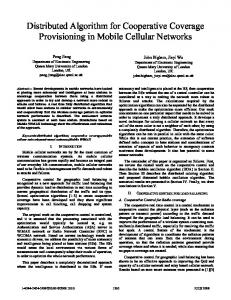
Both terms on the right-hand side in the previous equation are has a compact support. finite if the data distribution density Thus, the variance is finite. The unbiased estimate and bounded variance can guarantee that the distributed EM algorithm is a stochastic approximation to the standard EM algorithm with probability one [23]. V. SIMULATIONS A. Distributed EM Algorithm A sensor network with 100 nodes is used for simulation. The sensors are randomly placed in a square shown in Fig. 2. We take the communication distance in Fig. 2 as 0.8. This results in a connected graph with 356 edges and its . The connectivity can be verified maximum degree is . by finding that the rank of Laplacian matrix is 99 or . The obEach node has 100 data observations servations are generated from three Gaussian components distributed in Fig. 3. Each of the Gaussian components is a Gaussian density, which can represent environment data clusters. In the first 30 nodes (node 1 to node 30), 90% observations come from the first Gaussian component and other 10% observations evenly from the other two Gaussian components. In the next 40 nodes (node 31 to node 70), 80% observations come from the second Gaussian component and other 20% observations evenly from the other two Gaussian components. In

Fig. 4. Three estimated mean values using the standard EM algorithm in the network with 100 nodes.

the last 30 nodes (node 71 to node 100), 90% observations come from the third Gaussian component and other 10% observations evenly from the other two Gaussian components. For comparison, the standard EM algorithm is executed in a center unit using all data from 100 nodes in the first test. The standard EM algorithm is also conducted in each of nodes using only local data in the second test. Obviously, in the second test, each node will have a different estimated result. Finally, the distributed EM algorithm runs simultaneously in all nodes in the third test. The updating rate of the consensus filter is selected as where

(42)

which can satisfy the requirement (41). In the second test, each node uses the standard EM algorithm individually, i.e., only local data is used to estimate the mean parameters. The first estimated mean value from each

1162

Fig. 5. Three estimated mean values using distributed EM algorithm in the network with 100 nodes.

Fig. 6. Ranks of the Laplacian matrix and the number of edges.

vector in all 100 nodes are shown in Fig. 4 and they are very different. The second estimated mean value has a similar result and is ignored here for simplicity. Each estimated mean value has a smooth section, which represents reliable estimates of those nodes whose most observations come from the corresponding Gaussian component. Other nodes cannot properly estimate the parameters due to limited observations used. The first estimated mean vector in 100 nodes using the mean values from each distributed EM algorithm are shown in Fig. 5. It can be seen that the estimated mean values in all nodes approximate to their true values (the true values are 0.2, 0.4, and 0.7). The second estimated mean value has a similar result and is ignored here for simplicity. The network connection can be changed if the communication distance between nodes is changed. Fig. 2 corresponds to the communication distance 0.8 in our simulation. Different communication distances from 0 to 1 are used to test the algorithm performance. The ranks of the Laplacian matrix and the


number of edges are calculated for different connections and , where shown in Fig. 6. It is known that is the number of the connected components in a graph [27]. The ranks of the Laplacian matrix and the number of edges increase with the increase of the communication distance. The dropped links occur often in sensor networks. This test can simulate how the dropped links affect the algorithm performance. One of the estimated mean values from all 100 nodes against different connections is shown in Fig. 7. It can be seen that the estimated values gradually decrease and converge to a stable value with the increasing communication distance or more links. When the communication distance is larger than 0.8, the graph is connected (see the ranks in Fig. 6). For a connected graph, the consensus filter is stable, i.e., all nodes can achieve a common agreement eventually. Thus, the failures of nodes or dropped links do not affect the final estimation results as long as the graph is still connected. This can be seen from the flat part of the diagram when the distance is larger than 0.8. The same data set is used in the first test where the standard EM algorithm is run in a center unit and in the third test where the distributed EM algorithm is run in each of nodes. The normalized log-likelihood updating is illustrated in Fig. 8. The solid line generated by using the distributed EM algorithm in one of the nodes monotonically increases, i.e., the learning of the distributed EM algorithm is convergent. It can also be seen that the updating is slower than the dashed line generated by using the standard EM algorithm due to its stochastic approximation nature. The estimated Gaussian components are also illustrated in Fig. 9. The initial Gaussian components are the same and shown in the dotted circle. The estimated Gaussian components by the distributed EM algorithm are the solid ellipses. They are very close to the dashed ellipses estimated by using the standard EM algorithm in a center unit. The Old Faithful data set contains data about the date of the observation of a geyser in Yellowstone, the duration of an eruption, and the time between eruptions. Both the duration of eruptions and the time between eruptions have bimodal distributions. We use the sensor network with 100 nodes to estimate the distributions. The sensor nodes are distributed in the same way as in the above tests. In this test, they are organized into four groups and each group has 25 nodes. The data in the date set is also divided into four groups and each group has 55 data pairs. Then, each sensor group takes one of data groups as its observations. Both the standard EM and distributed EM algorithms are tested and results are illustrated in Fig. 10. The estimated results by the standard EM algorithm are shown as the solid ellipses. The estimated results of the tenth, 50th, and 90th node by the distributed EM algorithm are shown as the dotted, dashed, and dashed–dotted ellipses, respectively. As only part of data held in each sensor node, the estimated results by the distributed EM algorithm are not exactly the results of the standard EM algorithm. However, the consensus filter can diffuse the local statistics to the sensor network; the results are the approximations to the results by the standard EM algorithm. To test a large network, 900 nodes are used and distributed in . The communication distance is the same a squared area . This results in a connected graph with 11 987 as above


1163

Fig. 7. One estimated mean value using the distributed EM algorithm in the network with 100 nodes for different connected graphs. The communication distance ranges from 0.1 to 1.0 representing different connected graphs. One hundred nodes are numbered from 1 to 100.

Fig. 8. Log-likelihood changes during 15 iterations.

edges and its maximum degree is . The connectivity can be verified by finding that the rank of Laplacian matrix is 899. The data used and their distribution are the same as those in the network with 100 nodes. The estimated Gaussian components and the normalized log-likelihood updating are illustrated in Fig. 11. It can be seen that the convergent rate and estimated results are very close to the results of the network with 100 node in Figs. 8 and 9. B. Applying Distributed EM Algorithm to Particle Filter Particle filter is one of the widely used tracking algorithms due to its applicability to nonlinear and non-Gaussian dynamic systems. In a particle filter, a moving object is modeled as a

Fig. 9. Estimated Gaussian densities by the standard EM algorithm (dashed ellipses), the estimated Gaussian densities by the distributed EM algorithm (solid ellipses), and initial Gaussian densities (dotted circle).

simple Markov process, specified by their state transition probabilities. Observations about states of the moving object are modeled by their likelihood probabilities. The aim of the algorithm is to estimate the posterior probability density function (pdf). Particle filter is applied as a Monte Carlo approximation to posterior pdf, i.e., the posterior pdf is represented by a set of weighted samples (or particles) [29], [30]. However, it is difficult to be used in sensor networks due to the transmission of large number of particles. We propose to use a low-dimensional

1164


Fig. 11. Estimated Gaussian densities in the network with 900 nodes.

Fig. 10. Old Faithful data set (dots), the estimated Gaussian densities by the standard EM algorithm (solid ellipses), and three estimated results by the distributed EM algorithm (dotted, dashed, and dashed–dotted ellipses).

Gaussian mixture model (GMM) to describe the posterior probability distribution function. The GMM parameters rather than weighted particles are transmitted over the network. The distributed EM algorithm can be employed to estimate the GMM parameters because it can exchange local summary quantities of particles between neighbor nodes and estimate global summary quantities of all particles. The particle filter can sample particles from the estimated GMM. The particle filter using the distributed EM algorithm is given in the following algorithm. Algorithm 2: Distributed Particle Filter (DPF) Initialization:

Fig. 12. Tracking trajectory result in one of the sensor nodes: the true trajectory (solid line) and the estimated trajectory (dotted line). The estimated particles at the beginning and the end of tracking are represented by the black dots in one node.

Draw particles from the initial distribution and initializing particle weights, Importance sampling step: 1) calculate the local summary quantities ; 2) estimate iteratively the global statistics 3) sample particles from the estimated Gaussian mixtures; 4) calculate the predicted particles; 5) calculate the predicted observations; 6) update the importance weights; 7) normalize the importance weights.

;

Selection step:

A sensor network with 100 nodes is used for tracking simulation. The sensors are randomly placed in a square 5 m 5 m shown in Fig. 2. We assume that a moving has a state equation object (43) where

is the Gaussian noise with variance

, and

particles according to the importance Resample weights and initializing the importance weights.

This algorithm is a standard particle filter algorithm except steps 2) and 3). Step 2) is the proposed distributed EM algorithm (see Algorithm 1), which iteratively estimates a Gaussian mixture model. Step 3) is used to generate the particles according to the estimated posterior probability.

The state includes coordinates and speed vectors. is the discrete sampling time. The position of node is denoted coordinates . The observation equation is a sonarby its


Fig. 13. Circle tracking result in one of the sensor nodes: the true trajectory (solid line) and the estimated trajectory (dotted line). The estimated particles at the beginning and the end of tracking are represented by the black dots in one node.

1165

The posterior distribution GMM is assumed to have three Gaussian components. The parameter estimation in the EM algorithm is executed ten times between two consecutive observations. . Each of sensor nodes contains 50 The target starts from . particles and the particles are initially distributed around The 200–step tracking result in one of the sensor nodes is shown in Fig. 12. It can be seen that the estimated trajectory (dotted line) is very close to the true trajectory (solid line). The estimated particles at the beginning and the end of tracking are also shown in Fig. 12 (see the black dot clusters). They represent the variance changes from large cluster at the beginning to small cluster at the end. Next the target moving along a circle trajectory is simulated. . The proposed particle filter still uses Its initial position is the state equation (43) and the observation equation (44) to track this circle trajectory. Each of sensor nodes contains 50 particles . All other and the particles are initially distributed around parameters are the same as the above. The 600-step tracking result in one of the sensor nodes is shown in Fig. 13. It can be seen that the estimated trajectory (dotted line) can track the true trajectory (solid line). The variance decreases from large cluster at the beginning to small cluster at the end. The speeds in and directions during the tracking are shown in Fig. 14. They are both assumed to be zero at the beginning of the tracking. They converge to sin and cos functions required in the circle tracking. VI. CONCLUSION

Fig. 14. Estimated speed results in x and y directions of circle tracking in one of the sensor nodes.

like model, which can observe the distance and angle between and the moving object a sensor positioned in

(44) where presents the Euclidean distance between and . represents the angle between and . The are variances of Gaussian noises and

This paper proposed a distributed EM algorithm. The main contribution includes the proposed consensus filter, its performance analysis, and its application to distributed particle filter. This paper also contributes the convergent proof of the distributed EM algorithm via the stochastic approximation approach. The simulation tests justify the proposed EM algorithm and its performance. This distributed EM algorithm only needs information exchanges between neighbor sensor nodes. The global information can be diffused over the entire network through the local information exchanges. It is scalable because the adding of more nodes does not affect the algorithm performance. It is also robust as it can still produce the right results even if failures of some nodes occur. The consensus filter is a low-pass filter, which can smooth away the high-frequency noise caused by the estimation of the global summary quantities. Currently, the number of Gaussian components is given. We can also use a distributed algorithm to estimate this number. A well-fitted approach to the estimate of this number is the one proposed in [24]. ACKNOWLEDGMENT The author would like to thank the anonymous reviewers for their valuable comments. REFERENCES [1] I. Akyildiz, W. Su, and Y. Sankarasubramniam, “A surevy on sensor networks,” IEEE Commun. Mag., vol. 40, no. 8, pp. 102–114, Aug. 2002.

1166

[2] D. Estrin, R. Govindan, J. Heidemann, and S. Kumar, “Next century challenges: Scalable coordination in sensor networks,” in Proc. ACM/IEEE Int. Conf. Mobile Comput. Netw., Seattle, WA, 1999, pp. 263–270. [3] R. D. Nowak, “Distributed EM algorithms for density estimation and clustering in sensor networks,” IEEE Trans. Signal Process., vol. 51, no. 8, pp. 2245–2253, Aug. 2003. [4] Y. Sheng, X. Hu, and P. Ramanathan, “Distributed particle filter with GMM approximation for multiple targets localization and tracking in wireless sensor networks,” in Proc. 4th Int. Symp. Inf. Process. Sensor Netw., Los Angeles, CA, Apr. 2005, pp. 181–188. [5] R. Kamimura, “Cooperative information maximization with Gaussian activation functions for self-organizing maps,” IEEE Trans. Neural Netw., vol. 17, no. 4, pp. 909–918, Jul. 2006. [6] C. Constantinopoulos and A. Likas, “Unsupervised learning of Gaussian mixtures based on variational component splitting,” IEEE Trans. Neural Netw., vol. 18, no. 3, pp. 745–755, May 2007. [7] X. Nguyen, M. I. Jordan, and B. Sinopoli, “A kernel-based learning approach to ad hoc sensor network localization,” ACM Trans. Sensor Netw., vol. 1, no. 1, pp. 134–152, 2005. [8] S. Simic, “A learning theory approach to sensor networks,” IEEE Pervasive Comput., vol. 2, no. 4, pp. 44–49, Oct./Dec. 2003. [9] R. A. Jacobs, M. I. Jordan, S. J. Nowlan, and G. E. Hinton, “Adaptive mixtures of local experts,” Neural Comput., vol. 3, pp. 79–87, 1991. [10] M. I. Jordan and R. A. Jacobs, “Hierarchical mixtures of experts and the EM algorithm,” Neural Comput., vol. 6, pp. 181–214, 1994. [11] J. Zhang, “The mean field theory in EM procedures for Markov random fields,” IEEE Trans. Signal Process., vol. 40, no. 3, pp. 2570–2583, Mar. 1992. [12] G. Celeux, F. Forbes, and N. Peyrard, “EM procedures using mean field-like approximations for Markov model-based image segmentation,” Pattern Recognit., vol. 36, pp. 131–144, 2003. [13] A. Diplaros, N. Vlassis, and T. Gevers, “A spatially constrained generative model and an EM algorithm for image segmentation,” IEEE Trans. Neural Netw., vol. 18, no. 3, pp. 798–808, May 2007. [14] F. Zhao, J. Shin, and J. Reich, “Information-driven dynamic sensor collaboration for tracking applications,” IEEE Signal Process. Mag., vol. 19, no. 2, pp. 61–72, Mar. 2002. [15] R. Olfati-Saber, “Distributed Kalman filter with embedded consensus filters,” in Proc. 44th IEEE Conf. Decision Control, Dec. 12–15, 2005, pp. 8179–8184. [16] A. Dempster, N. Laird, and D. Rubin, “Maximum likelihood estimation from incomplete data via the EM algorithm,” J. Roy. Statist. Soc., vol. 39, pp. 1–38, 1977. [17] P. Gupta and P. R. Kumar, “The capacity of wireless networks,” IEEE Trans. Inf. Theory, vol. 46, no. 3, pp. 388–404, May 2000. [18] R. M. Neal and G. E. Hinton, “A view of the EM algorithm that justifies incremental, sparse, and other variants,” in Learning in Graphical Models, M. I. Jordan, Ed. Boston, MA: Kluwer, 1998, pp. 355–368.


[19] R. Olfati-Saber and J. S. Shamma, “Consensus filters for sensor networks and distributed sensor fusion,” in Proc. 44th IEEE Conf. Decision Control, Dec. 12–15, 2005, pp. 6698–6703. [20] W. Ren and R. W. Beard, “Consensus seeking in multiagent systems under dynamically changing interaction topologies,” IEEE Trans. Autom. Control, vol. 50, no. 5, pp. 655–661, May 2005. [21] L. Xu and M. I. Jordan, “On convergence properties of the EM algorithm for Gaussian mixtures,” Neural Comput., vol. 8, pp. 129–151, 1996. [22] M. Sato and S. Ishii, “On-line EM algorithm for the normalized Guassian network,” Neural Comput., vol. 12, no. 2, pp. 407–432, 2000. [23] H. J. Kushner and G. G. Yin, Stochastic Approximation Algorithms and Applications. New York: Springer-Verlag, 1997. [24] M. A. T. Figueiredo and A. K. Jain, “Unsupervised learning of finite mixture models,” IEEE Trans. Pattern Anal. Mach. Intell., vol. 24, no. 3, pp. 381–396, Mar. 2002. [25] N. A. Lynch, Distributed Algorithms. San Francisco, CA: Morgan Kaufmann, 1996. [26] R. Olfati-Saber and R. M. Murray, “Consensus problems in networks of agents with switching topology and time-delay,” IEEE Trans. Autom. Control, vol. 49, no. 9, pp. 101–115, Sep. 2004. [27] C. Godsil and G. Royle, Algebraic Graph Theory. New York: Springer-Verlag, 2001. [28] S. Boyd, P. Diaconis, and L. Xiao, “Fastest mixing Markov chain on a graph,” SIAM Rev., vol. 46, no. 4, pp. 667–689, Dec. 2004. [29] M. S. Arulampalam, S. Maskell, N. Gordon, and T. Clapp, “A tutorial on particle filters for online nonlinear/non-Gaussian Bayesian tracking,” IEEE Trans. Signal Process., vol. 50, no. 2, pp. 174–188, Feb. 2002. [30] A. Doucet, N. de Freitas, and N. Gordon, Sequential Monte Carlo Methods. New York: Springer-Verlag, 2001. Dongbing Gu (M’01–SM’07) received the B.Sc. and M.Sc. degrees in control engineering from Beijing Institute of Technology, Beijing, China, and the Ph.D. degree in robotics from University of Essex, Colchester, U.K., in 2004. He joined the Department of Electronic Engineering, Changchun Institute of Optics and Fine Mechanics, China, as a Lecturer in 1988, and became an Associate Professor in 1993 and a Professor in 1999. He was an Academic Visiting Scholar at the Department of Engineering Science, University of Oxford, Oxford, U.K., during October 1996 and October 1997. Since 2000, he has been a Lecturer at the Department of Computing and Electronic Systems, University of Essex. His current research interests include multiagent systems, wireless sensor networks, distributed control algorithms, distributed information fusion, cooperative control, reinforcement learning, fuzzy logic and neural-network-based motion control, and model predictive control.