Embedded Cartesian Genetic Programming and the Lawnmower and Hierarchical-if-and-only-if Problems Genetic Programming Track James Alfred Walker
[email protected]
Julian Francis Miller
[email protected]
Intelligent Systems Group, Department of Electronics University of York, Heslington, York, YO10 5DD, UK
ABSTRACT Embedded Cartesian Genetic Programming (ECGP) is an extension of the directed graph based Cartesian Genetic Programming (CGP), which is capable of automatically acquiring, evolving and re-using partial solutions in the form of modules. In this paper, we apply for the first time, CGP and ECGP to the well known Lawnmower problem and to the Hierarchical-if-and-Only-if problem. The latter is normally associated with Genetic Algorithms. Computational effort figures are calculated from the results of both CGP and ECGP and our results compare favourably with other techniques.
Categories and Subject Descriptors I.2.2 [Artificial Intelligence]: Automatic Programming— Program synthesis; I.2.8 [Artificial Intelligence]: Problem Solving, Control Methods and Search
shown ECGP to be more computational efficient than CGP on evolving solutions to a range of digital circuit problems (such as even parity, adders and multipliers) and that the speedup grows with problem difficulty. This suggests that ECGP may be even more computational efficient than CGP on harder problems. The aim for this paper is to build on the results from the previous work on ECGP, by applying the technique to two problems that are not related to circuit evolution. The two problems chosen are: the lawnmower problem, which is a well known problem in the GP community and the Hierarchical if-and-only-if (H-IFF) problem, which is normally associated with Genetic Algorithms. The plan for the paper is as follows: Section 2 is an overview of related work. In section 3 we describe ECGP and compare it with CGP. The details of our experiments, including descriptions of the lawnmower and H-IFF problems are shown in section 4 followed by the results and comparisons for both experiments in section 5. Section 6 gives conclusions and some suggestions for future work.
General Terms Algorithms, Design, Performance
Keywords Cartesian Genetic Programming, Embedded Cartesian Genetic Programming, Module Acquisition, Automatically Defined Functions, Evolution, Lawnmower problem, Hierarchical-if-and-only-if
1.
INTRODUCTION
Embedded Cartesian Genetic Programming (ECGP) is an extension of the directed graph-based Cartesian Genetic Programming (CGP), incorporating ideas from a technique known as Module Acquisition [1]. This allows the automatic acquisition, evolution and re-use of partial solutions in the form of modules. Previous work [15, 17, 16] has
Permission to make digital or hard copies of all or part of this work for personal or classroom use is granted without fee provided that copies are not made or distributed for profit or commercial advantage and that copies bear this notice and the full citation on the first page. To copy otherwise, to republish, to post on servers or to redistribute to lists, requires prior specific permission and/or a fee. GECCO’06, July 8–12, 2006, Seattle, Washington, USA. Copyright 2006 ACM 1-59593-186-4/06/0007 ...$5.00.
2.
MODULE ACQUISITION, AUTOMATICALLY DEFINED FUNCTIONS AND M-ACROS
Module Acquisition [1] adds two operators to the evolutionary process, compress that selects a section of the genotype to make it immune to manipulation from operators (the module) and expand which decompresses a module in the genotype therefore allowing this section of the genotype to be manipulated once more. The fitness of a genotype is unaffected by these operators. Module Acquisition allows the possibility of having modules within modules. These techniques have been shown to decrease the time taken to find a solution. Rosca’s method of Adaptive Representation through Learning (ARL) [11] also extracted program segments that were encapsulated and used to augment the GP function set. However, Dessi et al [3] showed that random selection of program sub-code for re-use is more effective than Roscas method across a range of problems. Once the contents of modules are themselves allowed to evolve (as in ECGP) they become a form of Automatically Defined Function, however in contrast to Koza’s form of Automatically Defined Functions [6] and Spector’s Automatically Defined Macros [13], there is no explicit specification of the number of or the internal structure of such modules. This freedom does exist in Spector’s PushGP [14].
CGP genotype:
6:2 0:0 0:0 0:0
020 213 3
4
1 50
2 51 50 50
51
52 o0
Same CGP genotype represented as an ECGP genotype:
0:0 2:0 0:0
2:0 1:0 3:0
3
4
Move
1:0 50:0 51
2:0 51:0 50:0
50:0
52
o0
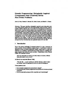
Figure 1: Examples of evolved CGP and ECGP genotypes for H-IFF problem with an 8-bit string (3 inputs, 1 output). For each node, the underlined gene encodes the function and the node type (only the function in CGP). The remaining genes encode the node inputs. Every node encoded in the CGP genotype represents a single output primitive function, therefore every node encoded in the ECGP genotype is of node type 0, and the second integer of each pair encoding the node inputs is always 0. The node index is underneath each node.
3. 3.1
1:0 2:0
3
EMBEDDED CARTESIAN GENETIC PROGRAMMING (ECGP)
5
0:0 1:0 4:0
2:0 3:1 5:1
2:0 3:0 7:0
8:0
6
7
8
oA
Module 6
0
3
1
Module 6 5
Turn
6:2 0:0 0:0 0:0
4
Prog n 7
Prog n
Output 8
V8A Randn 2
Frog
6 4
Figure 2: An ECGP genotype and corresponding phenotype for the 8-bit H-IFF problem. The underlined genes encode the function and node type of each node. The function lookup table is: v8a(0), frog (1), progn(2). See section 4.2 for details. The index labels are shown underneath each program input and node in the genotype and phenotype. Module 6 represents a possible structure for a subroutine constructed from the function set. The inactive areas of the genotype and phenotype are shown in grey dashes (nodes 4 and 6).
Representation
ECGP and CGP share the same structure and represent a program as a directed graph (that for feed-forward functions is acyclic). The benefit of this type of representation is the implicit re-use of nodes in the directed graph. The genotype is a list of integers that encode the connections and functions of each node of the directed graph. CGP used a program topology defined by a rectangular grid of nodes with a user defined number of rows and columns. However, later work in CGP always chose the number of rows to be one, thus giving a one-dimensional topology. This is always used in ECGP. In CGP, the genotype is a fixed length representation (in terms of nodes and genes). However, in ECGP the genotype is a variable length representation (in terms of nodes and genes), in which the number of nodes and genes in the graph can vary but is bounded. The number of nodes in the ECGP genotype vary as a result of the compression and expansion of modules. Also, the number of genes vary as a result of the re-use of modules elsewhere in the genotype, and the module mutation operators changing the number of node inputs. Despite the differences, both genotypes decode into a bounded variablelength directed graph (phenotype), as not all of the nodes encoded in the genotype have to be connected. This allows areas of the genotype to be inactive and have no influence on the phenotype, leading to a neutral effect on genotype fitness called neutrality. This unique type of neutrality has been investigated in detail [7] and found to be extremely beneficial to the evolutionary process on the problems studied. In Figure 1 an example of the differences between a CGP and an ECGP genotype are shown. All of the ECGP genotypes in the initial population have the same number of nodes and genes, and every node represents a primitive function (no modules are present). Each of the nodes consist of a number of genes. In ECGP, each gene consists of a pair of integers, as opposed to a sin-
gle integer in CGP. The first integer pair of each ECGP node encodes the primitive function (as in CGP) or module (by their unique identifier) that the node represents and the node type (introduced in ECGP). Node types allow the identification of nodes encoded in the genotype which represent: primitive functions (node type 0), modules that contain an original section of the genotype (node type I) and modules that contain a re-used section of the genotype (node type II). Different node types need to be identified, as operators act differently on the nodes encoded in the genotype depending on their node type (further details are explained in section 3.3). The remaining integer pairs in each ECGP node encode the node inputs. The first integer in each pair encodes the node index in the genotype or program input (terminal), whilst the second integer encodes the output of the node (nodes can have multiple outputs in ECGP). The number of inputs and outputs that a node has is dictated by the arity of its function. The nodes take their inputs in a feed forward manner from either the output of a previous node or from a program inputs (terminals). The program inputs are labelled from 0 to n-1 where n is the number of program inputs. The nodes in the genotype are also labelled sequentially starting from n to n+m-1 where m is the user-determined upper bound of the number of nodes. If the problem requires k program outputs then k integers are added to the end of the genotype, each one encoding a pointer to the output of a node in the graph where the program output is taken from. These k integers are initially set as pointers to the outputs of the last k nodes in the genotype. Figure 2 shows an ECGP genotype and its corresponding phenotype (a 8-bit H-IFF problem), whilst Figure 3 illustrates the decoding process of the genotype. Both CGP and ECGP use a (1 + 4) evolutionary strategy as defined below:
Step 1:
6:3:4:2 0:0 0:0 1:0 1:0 1:0 1:0 3:0 0:0 3:0 2:0
6:2 0:0 0:0 0:0 3
1:0 2:0 4
6:2 0:0 0:0 0:0
0:0 1:0 4:0
2:0 3:1 5:1
2:0 3:0 7:0
8:0
6
7
8
oA
0:0 1:0 4:0
2:0 3:1 5:1
2:0 3:0 7:0
8:0
6
7
8
oA
5
3
4
5
6
3:0
6:0
oA
oB
Step 2: 6:2 0:0 0:0 0:0 3
1:0 2:0 4
6:2 0:0 0:0 0:0 5
Step 3: 6:2 0:0 0:0 0:0 3
1:0 2:0 4
6:2 0:0 0:0 0:0
2:0 3:1 5:1
2:0 3:0 7:0
8:0
6
7
8
oA
1
0:0 1:0 4:0
2:0 3:1 5:1
2:0 3:0 7:0
8:0
Module Input C
6
7
8
oA
5
3
1:0 2:0 4
6:2 0:0 0:0 0:0 5
Figure 3: Decoding the ECGP genotype from Figure 2. Step 1: Output A (oA ) connects to the output of node 8, move to node 8. Step 2: Node 8 connects to the output of nodes 3 and 7, move to nodes 3 and 7. Step 3: Nodes 3 and 7 connect to the output of nodes 3 and 5, and program input 0, move to node 5 (as node 3 has already been processed). Step 4: Node 5 only connects to program input 0, therefore the genotype is now decoded.
Module Output A
V8A
0 Module Input B
0:0 1:0 4:0
Step 4: 6:2 0:0 0:0 0:0
Module Input A
3
Frog 5
Frog 4
Module Output B
V8A 6
2
Figure 4: The genotype and corresponding phenotype of a module 6 from Figure 2. The first section of the genotype is the module header. For each node, the underlined genes encode the function, the remaining genes encode the node inputs. The function lookup table is: v8a(0), frog (1), progn(2). The index labels are shown underneath each module input and node in the genotype and phenotype.The inactive areas of the genotype and phenotype are shown in grey dashes. The dotted box represents the edges of the module.
1. Randomly generate an initial population of 5 genotypes and select the fittest. 2. Carry out point-wise mutation on the winning parent to generate 4 offspring. 3. Construct a new generation with the winner and its offspring. 4. Select a winner from the current population using the following rules: (a) If any offspring has a better fitness; the best becomes the winner. (b) Otherwise, an offspring with the same fitness as the best is randomly selected. (c) Otherwise, the parent remains as the winner. 5. Go to step 2 unless the maximum number of generations is reached or a solution is found.
3.2
Module Representation
A module is represented as a bounded variable length genotype that has the same characteristics of a ECGP genotype. The module genotype consists of a list of integers and is split into two parts: the module header and the module body. The module header contains four integers and stores information about the module. Each of the four integers encodes the module identifier, the number of module inputs, the number of nodes contained in the module and the number of module outputs respectively. The module body encodes the connections and functions of the nodes contained in the module and the module outputs (similar to program outputs), in the same way as any ECGP genotype. An example of a module genotype showing the separate components is shown in Figure 4, where the first block of the module genotype consisting of four numbers represents the module header. The nodes are represented in the same manner as ECGP and the module outputs encode which nodes in the module the outputs are taken from.
The size of a module genotype is determined by the number of nodes and module outputs that it encodes. The number of nodes encoded in the module genotype is bounded between a minimum limit of two (any fewer and it would either be an empty module or a primitive function) and a maximum limit that is set by the user. Likewise, the number of module outputs encoded in the module genotype is also bounded between a minimum limit of one (otherwise there would be no way to connect to the module and access its result to the given inputs) and a maximum of p module outputs, where p is equal to the number of nodes contained in the module (one module output per node). The number of module inputs that a module is allowed to have is also restricted between a minimum of two and a maximum of 2p module inputs. However, the number of module inputs allowed does not affect the size of the module genotype, as they are not encoded in the module genotype. In its current form, ECGP only allows modules to contain nodes representing primitive functions rather than nodes representing other modules. Once a module is created, the module genotype is stored in the module list, which is an extension of the primitive function list. This allows any node in the genotype of an individual to be mutated into any module or primitive function present in either of these lists for that generation. The module list is dynamic and has no restrictions on its maximum size and is updated every generation when the fittest individual (chosen in accordance with the evolutionary strategy used in Section 3.1) in the generation is promoted to the next generation (i.e. the next generation inherits the module list of the fittest individual in the previous generation). This creates a regulatory control of the size of the module list, so that it does not grow beyond a certain size. The nodes contained inside the module are not necessarily connected and are immune from the main genotype point mutation operator. However, the module itself is allowed to be mutated by the module mutation operators (see Section 3.3).
3.3
Operators
ECGP extends CGP by allowing the use of dynamic acquisition, evolution and the re-use of modules. This is achieved through extra mutation operators, which are used in conjunction with the genotype point mutation of CGP. The compress operator constructs modules by selecting two random points in the genotype (in accordance with the rules for the module size restrictions) and encapsulates all the nodes (of type 0) between these two points into a new module, which is encoded into a module genotype as described earlier. Note, that if there any nodes of type I or II between the two selected points, the compress operator does not take place (this is because at present we do not allow modules within modules). The number of module inputs a module is initialized with, is determined by the number of connections between the inputs of the nodes that are going to be encapsulated into a module, and the outputs of any previous nodes or program inputs (terminals) in the genotype, when the module is created. Likewise, the number of module outputs possessed by a module is determined by the number of connections between the inputs of the latter nodes in the genotype and the outputs of the nodes that are going to be encapsulated in the module, when it is created. Any module created by the compress operator is represented in the genotype as a type I node. The gene representing the function and node type in any type I node is immune from the genotype point mutation operator therefore allowing the type I node to remain in the genotype of an individual until it is removed by the expand operator. The expand operator destroys a type I node by replacing it in the genotype with the nodes contained in the module, which the type I node represented. The inputs of the latter nodes in the genotype are updated in the final stage of both the compress and expand operators, so all the connections remain intact. The compress and expand operators only make a structural change to the genotype and have no affect on genotype fitness, as the genotype before and after the action of these operators represent the same directed graph. The expand operator has twice the probability of being applied to the genotype than the compress operator. We found that this introduces a pressure for good modules to replicate quickly in the genotype of an individual in order to survive. This can be seen as survival-of-the-fittest modules within the genotype itself. Modules can replicate within a genotype through the action of the genotype point mutation operator. This is identical to the operator used in CGP, except it can mutate the function of a node (of type 0 or II) to any of the primitive functions or any available modules in the module list. If a node is mutated to represent a module, it is classed as a type II node. The genotype point mutation operator can also mutate the function of a type II node to any of the predefined functions or any available modules in the module list. It can also mutate any of the inputs of a type II node in the same way it would mutate the inputs of a type 0 node. If the function of a type 0 or type II node is mutated, the new node keeps however many of the original nodes inputs it needs, and randomly generates any extra inputs it requires. Type II nodes are also immune from the expand operator, as this could cause excessive growth of the genotype that could possibly lead to bloat. To summarize the properties of node types 0, I and II are shown in Table 1. A module can be represented by two node
Table 1: The three nodes types and how the operators effect each of them Node Action of Action of Action of Genotype Type Compress Expand Point Mutation Compress Changes function 0 Immune into module or inputs Expand I Immune Changes inputs into nodes Changes function II Immune Immune or inputs
types (node type I and II) in order to reduce the excessive growth of the genotype and to induce a selection pressure on the modules. Therefore, the modules have to replicate in the genotype (make the transition from being represented by a type I to a type II node) and be associated with a high fitness genotype in order to survive. Once the module is represented by a type II node it is harder for the module to be removed from the module list, as it has a lower probability of being removed from the genotype (as it cannot be expanded). This is advantageous as it allows good modules to stay in the module list, but it is also disadvantageous as it could possibly allow the evolution of the genotype to progress at a slower rate. The module genotypes contained in the module list can also be evolved through the action of five different operators: module point mutation, add-input, add-output, remove-input and remove-output. The module point mutation operator is a restricted version of the ECGP genotype point mutation operator, as it can still mutate the inputs and function of any node encoded in the module genotype, but it is not allowed to introduce any type II nodes into the module genotype. It can also mutate which node output each of the module outputs are connected to (similar to program outputs in CGP). The add-input and add-output operators allow greater connectivity to and from the contents of a module, by increasing the number of module inputs or module outputs by one respectively each time either operator is applied, making a more generalized module. When the add-input operator is applied to a module, the gene representing the number of module inputs in the module header is incremented by one, and an extra gene is inserted into all nodes (type I and type II) representing the module in the genotype, as a randomly chosen value for the new module input. Likewise, when the add-output operator is applied to a module, the gene representing the number of module outputs in the module header is incremented by one, and an extra gene is added to the module output section of the module genotype, as randomly chosen values for the node index and node output that the new module output is connected to. Alternatively, the remove-input and remove-output operators reduce the connectivity to and from the contents of a module, by decreasing the number of module inputs or module outputs by one respectively each time either operator is applied, therefore making a more specialized module. When the remove-output operator is applied to a module, the gene representing the number of module inputs in the module header is decremented by one, and the gene corresponding to the module input randomly chosen, is removed from all nodes (type I and type II) representing the module in the genotype. Likewise, when the remove-output operator is applied to a module, the gene representing the number
of module outputs in the module header is decremented by one, and the gene corresponding to the randomly chosen module output is removed from the module output section of the module genotype. All of the operators: add-input, add-output, remove-input, and remove-output must comply with the restrictions on the number of module inputs and module outputs at all times. Further information about all of the module operators (including figures explaining their operation) is available in our previous work [15, 17, 16].
4.
4.1
1101-100 1101 11
Lawnmower Problem
The Lawnmower Problem was first introduced by Koza in his second book [6] to test the effectiveness of Automatically Defined Functions by exploiting the modularity of the lawnmower problem. Since then it has been used as a benchmark problem by many other researchers in the testing of new GP techniques and representations [9]. The concept of the lawnmower problem is to guide a lawnmower around a grass lawn, which consists of n x m squares (where n and m are user defined parameters). The lawnmower moves around the lawn one square at a time, and cuts all the grass in each square it visits. The lawnmower is allowed to revisit a square of the lawn as many times as it likes, but the grass in a square can only be cut by the lawnmower once, therefore by revisiting squares of the lawn, the lawnmower is using an inefficient approach to mowing the lawn. However, the lawn is a ”magic” lawn, when the lawnmower moves off a square on any side of the lawn, it reappears in the square on the opposite side of the lawn. The lawnmower always starts in the centre square of the lawn and starts off by facing in a northward direction. The lawn is cut when every square has been visited by the lawnmower. The movement of the lawnmower is controlled by a CGP or ECGP program. The program has three inputs which it can use: move, which moves the lawnmower one square forward on the lawn in the direction the lawnmower is facing, and cuts all of the grass in that square, turn, which rotates the lawnmower 90◦ clockwise in the current square on the lawn and random constant, which stores a randomly distributed vector for the entire run of the form [x, y], where 0