Recurrent Cartesian Genetic Programming Applied to Series Forecasting Andrew James Turner
Julian Francis Miller
The University of York Department of Electronics YO10 5DD, UK
The University of York Department of Electronics YO10 5DD, UK
[email protected] ABSTRACT Recurrent Cartesian Genetic Programming is a recent proposed extension to Cartesian Genetic Programming which allows feedback and cyclic program structures to be evolved. We apply both standard and Recurrent Cartesian Genetic Programming to the domain of series forecasting. Their performance is compared to a number of well-known classical forecasting approaches. Our results show that not only does Recurrent Cartesian Genetic Programming outperform standard Cartesian Genetic Programming, but it also outperforms many standard forecasting techniques.
Keywords Genetic programming, Forecasting
1.
INTRODUCTION
Cartesian Genetic Programming (CGP) [2, 3] is a Genetic Programming (GP) [4] method which represents computational structures as directed acyclic graphs. This brings many advantages over the more commonly used tree structure. For instance: CGP is naturally suited to multipleinput multiple-output (MIMO) tasks, it allows internally calculated values to be reused many times, it benefits from explicit neutral genetic drift and does not suffer from program bloat. It has recently been shown that with minor changes to the encoding, CGP can also encode cyclic graphs. The extended form of CGP is called Recurrent Cartesian Genetic Programming (RCGP) [6, 7]. Allowing recurrent connections enables RCGP phenotypes to hold internal states based on previous inputs. This enables RCGP to be applied to partially observable tasks such as those which require memory or feedback. This paper applies both standard CGP and RCGP for the first time to series forecasting. Series forecasting is an important machine learning domain finding application in many disciplines including: economics, politics and planning. Although previously alternative types of GP have been applied
Permission to make digital or hard copies of all or part of this work for personal or classroom use is granted without fee provided that copies are not made or distributed for profit or commercial advantage and that copies bear this notice and the full citation on the first page. To copy otherwise, to republish, to post on servers or to redistribute to lists, requires prior specific permission and/or a fee. GECCO’15, July 11-15, 2015, Madrid, Spain. Copyright 2015 ACM TBA ...$15.00.
[email protected] to series prediction, these results are not used here for comparisons. This is due to the many differences in benchmark implementation used, making any comparisons less valid. Here we compare CGP and RCGP to many standard forecasting methods ourselves using the same, well specified, formation of the benchmarks ensuring a fair comparison. The work compares CGP and RCGP to a range of standard forecasting techniques comprising Random Walk forecasting (RWF), MEAN, Exponential smoothing (ETS) and Autoregressive integrated moving average (ARIMA). Comparing new forecasting methods with two naive and two complex standard methods (including ARIMA) is the recommended methodology of Richard Hyndman, a recognized expert in the field of forecasting, when evaluating new forecasting methods; http://robjhyndman.com/ hyndsight/benchmarks/. The Forecast package [1] implementation was used for RWF, MEAN, ETS and ARIMA.
2.
RECURRENT CARTESIAN GENETIC PROGRAMMING
Recurrent Cartesian Genetic Programming (RCGP) [6, 7] is a recent extension to CGP [2] which allows both acyclic and recurrent connections. In regular CGP, connection genes are restricted to only allow nodes to connect to previous nodes in the graph; including inputs. In RCGP this restriction is lifted so that it allows connections genes to connect a given node to any node, including itself, or program inputs. Once the acyclic restriction is removed, RCGP phenotypes can contain recurrent connections. The level of recurrence present in RCGP is biased using a recurrent connection probability. This parameter controls the probability that when a connection gene is mutated it will result in a recurrent connection. This parameter does not however limit the maximum / minimum number of recurrent connections; except for values of 0% and 100%. RCGP chromosomes are executed identically to standard CGP chromosomes. The inputs are applied, each active node is updated once in order of node index, and the outputs read. The next set of inputs are then applied and the process repeated. The difference with RCGP is that the program output(s) can be determined by the current inputs and the state of the internal nodes. One important aspect of RCGP, again described in [6], is that it is now possible for node output values to be read before they have been calculated. For this reason all nodes are initialised to output zero until they have calculated their own output value.
3.
In this paper CGP and RCGP are applied to series forecasting using a recursive forecasting method. This method involves making previous forecasts available as inputs to be used for subsequent forecasts; determined by the embedding dimension of the training data. This allows for forecasts up to arbitrary horizons. The fitness function used by CGP and RCGP represents how well the solutions recursively predict sections of the training data. This is achieved by recursively predicting the next fifty samples from t = 50, t = 100,..., t = 950; the forecasts start from t = 50 and not t = 0 as a number of previous values are required to make the initial forecasts. The fitness awarded to each chromosome is the mean square error between the correct and produced forecasts. Unlike CGP, when using RCGP the output of the programs are a function of the current inputs and the current state of the network. This means the network must be ‘primed’ before it can be used to make forecasts. The priming process is to apply previous observed values to the network, in sequence, and execute the phenotype in each case. The outputs are not used. This causes the internal nodes to calculate suitable values/states before forecasting begins. Here when using RCGP the previous 50 samples from each starting point are applied to the network before making future predictions. A validation scheme is also used to prevent over-training. Generalisation is assessed by recording how well the solutions perform beyond the forecast horizon used during training. Starting at t = 100, t = 200, ..., t = 900 forecasts are made up to a horizon of 100 samples. The mean square error of the forecasts between a horizon of 50 samples and 100 samples are then used as a validation fitness score. The chromosome which achieves the best validation score is then retained once the maximum number of generations has elapsed and used as the final solution. In the work presented here CGP and RCGP use the following “off-the shelf” parameters: (1+4)-ES, 10000 generations, 3% probabilistic mutation, 100 nodes, and a node arity of 2. In the case of RCGP a 10% recurrent connection probability is used. In both cases the function set contains: +, −, ∗, /, sin, cos, exp and log.
4.
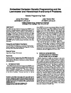
Table 1: MSE achived by the Forecasting methods.
APPLICATION TO FORECASTING
EXPERIMENTS
Here three standard benchmarks are utilised to assess the effectiveness of using CGP and RCGP as forecasting techniques. In all cases 1000 samples are used for training and 100 for testing. Additionally in all cases the series are normalised into the range [0,1]. The benchmarks comprise, laser, Makey-Glass and sunpots. The laser benchmark is available at [8]. The Mackey-Glass benchmark is created from Equation 1 using a = 0.2, b = 0.1, c = 10 and τ = 17, x(t) = 0 when t ≤ 0. A series is produced using fourth order Runge-Kutta integration with a time step of dt = 0.01 seconds. This series is then sampled once a second to produce the series used as the benchmark. The first 117 seconds (samples) are removed to avoid the transient response time. Then the following 1100 seconds (samples) are used for the training and testing sets. Finally, the smoothed monthly sunspots benchmark, available from [5], from November 1834 to June 1926.
Method RWF MEAN ETS ARIMA CGP RCGP
Laser 0.034227 0.027151 0.034223 0.034148 0.027091 0.004424
Mackey-Glass 0.109334 0.067324 0.357603 0.071481 0.058746 0.025706
Sunspots 0.176262 0.034399 0.546006 0.034972 0.026894 0.011922
dx(t) a · x(t − τ ) = − b · x(t) dt 1 + xc (t − τ )
(1)
The results of applying the forecasting techniques on the testing data are given in Table 1. In the case of RWF, MEAN, ETS and ARIMA only one model is created and so the performance of that model is given. In the case of CGP and RCGP, 50 runs of training were carried out. The results given are the results from the run which achieved the best validation score. This is representative of how CGP and RCGP would be applied in a real world application.
5.
CONCLUSIONS
This paper has demonstrated how CGP and RCGP can be applied towards series forecasting. From the comparisons with standard forecasting methods it has been shown that CGP and RCGP represent powerful forecasting methods worthy of further investigation. Finally, it has also been shown that the ability of RCGP to create recurrence in the evolved solutions represents a major advantage over standard feed-forward CGP in the domain of series forecasting.
6.
REFERENCES
[1] R. J. Hyndman, G. Athanasopoulos, S. Razbash, D. Schmidt, Z. Zhou, Y. Khan, C. Bergmeir, and E. Wang. forecast: Forecasting functions for time series and linear models, 2014. R package version 5.4. [2] J. F. Miller, editor. Cartesian Genetic Programming. Springer, 2011. [3] J. F. Miller and P. Thomson. Cartesian genetic programming. In Proceedings of the Third European Conference on Genetic Programming (EuroGP), volume 1820, pages 121–132. Springer-Verlag, 2000. [4] R. Poli, W. W. B. Langdon, N. F. McPhee, and J. R. Koza. A field guide to Genetic Programming. Published via http://lulu.com and freely available at http://www.gp-field-guide.org.uk, 2008. [5] SIDC-team. The International Sunspot Number. Monthly Report on the International Sunspot Number, online catalogue, 1700-1987. [6] A. J. Turner and J. F. Miller. Recurrent Cartesian Genetic Programming. In 13th International Conference on Parallel Problem Solving from Nature (PPSN 2014), volume 8672 of LNCS, pages 476–486, 2014. [7] A. J. Turner and J. F. Miller. Recurrent Cartesian Genetic Programming Applied to Famous Mathematical Sequences. In Proceedings of the Seventh York Doctoral Symposium on Computer Science & Electronics, pages 37–46, 2014. [8] A. Weigend. Santa fe competition data sets, July 2014.