EMBEDDED HARDWARE ARCHITECTURE FOR STATISTICAL RAIN FORECAST Tassilo Meindl, Walter Moniaci, Davide Gallesio, Eros Pasero Polytechnic of Turin, Neuronica laboratory, Corso Duca degli Abruzzi, I-10129 Turin, Italy E-mail:
[email protected]
Weather forecasts are a typical problem where a huge amount of data coming from different types of sensors must be elaborated by means of complex, time consuming algorithms. In this paper we present a new embedded data mining system, based on a FPGA [1], which performs statistical data elaboration on sensorial data and provides nowcasting for the next one, two and three hours. The statistical algorithm has been tested for forecasts of temperature, humidity and rain and provides promising results.
1. INTRODUCTION Weather forecast systems are among the most heavy equation systems that a computer must solve. A very large amount of data, coming from satellites, synoptic stations and sensors located around our planet give each day information that must be used to foresee the weather situation in next hours and days all around the world. Weather reports give forecasts for next 24, 48 and 72 hours for wide areas. Today they are quite reliable but it is not unusual that in a restricted region the conditions suddenly change. Snow, ice and fog are very dangerous events that can occur on the roads giving important problems for road safety. So whereas a traditional weather forecast system provides a powerful system able to give indications about the weather evolution in next days in a large area, this embedded system is used to make very short-term local prediction and warning decisions. This is made possible thanks to a powerful suite of detection and prediction algorithms. The usefulness of this approach is that the knowledge of the next three hours weather conditions, for example, can be used to organize outdoor activities. For example the knowledge about a rain event in next two hours can be used to choose the right set of tires in a formula one competition. The knowledge of fog occurrence in next three hours allows the airport maintenance staff to take in advance important decisions in order to avoid canceling flight at the last minute. The realization of an autonomous embedded portable weather station that can be used without a PC, able to predict microclimate meteorological events and alarms in restricted areas within short time is therefore an interesting and useful approach different from the classical macroclimate meteorological forecast systems.
2. HARDWARE ARCHITECTURE We propose a new hardware architecture for embedded data processing of sensorial data. In order to increase the field of possible applications a distributed hardware architecture has been realized. Data Management and Controlling Real Time Clock
Data Processing
32.768 kHz
Onboard Sensors
433 MHz Radio Transceiver
Cygnal 8051 Microcontroller
LCD Display
USB
In System Programming
ABSTRACT
Control
2mbit Program Flash
24 MHz
XILINX Spartan 3 FPGA
4mbit Data Flash
Power Supply Network
Battery Embedded Data Processing Station
Wireless Sensors
PC
Figure 1. Embedded Data Processing Station. The system as shown in figure 1 is primarily based on a microcontroller, which is the heart of the “Data Management and Controlling” part, and a FPGA connected to several memory blocks, which constitutes the “Data Processing” part. The simple and fast modifiability of the microcontroller’s firmware, allows for an efficient acquisition of sensorial data and the time stamp, and provides user interfaces, including the connection to a PC or the on-board buttons and display, whereby the elaboration of data and the prevision algorithm has been implemented completely in the FPGA. The exact timing is one of the key points for data processing of sensorial data in order to guarantee data consistency whilst not saving time stamps into the data memory. Every 15 minutes the microcontroller performs data acquisition from the sensors, which are displayed directly to the user by a LCD display. The FPGA performs the statistical algorithm described in the next section and saves the forecast values for the next 1, 2 and 3 hours into a data register, which can be read by the microcontroller. During operation on battery in the absence of powering from the USB connector, the microcontroller performs efficient power management.
The FPGA core has been implemented completely using VHDL. Interfacing to the external components and the controlling part has been implemented directly in VHDL, whilst the statistical processing part has been implemented using CODESIMULINK, a MATLAB tool developed at the Polytechnic of Turin, which automatically generates a synthesizable VHDL code.
3. ALGORITHM DESCRIPTION The algorithm is composed of a “Best Day Calculation” and the forecast module. The “Best Day Calculation” module searches in the historical database the day which matches best the current day, based on the last four hour measures of a particular parameter selected by the Parzen method [4]. The gradient evolution of the historical data allows then the Forecast module to perform a simple data prevision for the next 1, 2 and 3 hours. The rain prediction is not an easy problem to solve. In fact rain is not a stationary phenomenon and the classical Auto Regressive eXogenous [3] model (ARX) does not provide good results. In this paper a new approach, based on statistical non parametric method, is shown. First we have to decide the variables that have more influence on the rain event. We used the Parzen method to establish the correlation among rain and other meteorological variables.
3.1 Parzen method The goal is to choose the best “predictors” for the rain forecast. We define the entropy of the parameters in the following way:
e(x) = − ∫ log ( p(x )) ⋅ p(x )dx +∞
−∞
(1)
In this formula p(x) is the Probability Density Function (PDF) of a random variable x. e(x) is an index of dispersion that lies in the range ]-∞,+∞[. Let Z be the vector of all the possible predictors that can be used to foresee the variable y (predictand). Now let X1 and X2 be two particular subsets of predictors taken from Z. The number of elements in X1 and X2 has to be the same. In order to establish the best set of predictors between X1 and X2 we calculated the following entropy difference:
d ( X , y ) = e ( X , y ) − e (x )
= − ∫ log P ( X , y ) ⋅ P( X , y )dXdy +
(2)
+ ∫ log P( X ) ⋅ P ( X )dX
where P(X,y) is the joint PDF of X and y and P(X) is the PDF of X (the predictors). Both PDFs are unknown and therefore it’s impossible to evaluate the integrals in (2). We circumvented this problem by estimating the unknown PDFs through the Parzen method. This method estimates the unknown probability density functions making a sum of Gauss kernels, each one centered on a record of the database. The formula is the following:
PX∗ ( X ; D , Λ) =
(
x j − xij 1 n m 1 ⋅ exp− ∑∏ 2 n i =1 j =1 2πλ 2λ2j j
)
2
(3)
where, • •
D = {X1, …, Xn}: is the data vector n: database dimension (number of records) xi,xij: these are the j-th component of X and Xi • • Λ: standard deviation vector, Λ= ( λ1,….,λm) Each standard deviation in Λ regulates the resolution of the estimator along the corresponding dimension. In its turn this allows us to estimate d(X1,y) and d(X2,y). The best between X1 and X2 is the one that gives rise to the smallest entropy difference. In the case shown in this paper the sets Xi are the data of the following meteorological variables: • Air temperature • Relative humidity • Solar radiation • Ground temperature • Atmospheric pressure At the end of the Parzen simulation we obtain that the most important meteorological variable for rain prediction is air relative humidity. Then we have to decide how many air relative humidity data in the past are necessary to have an affordable forecast. We use again the Parzen method and it is put in evidence that the last 4 hour humidity values are sufficient to make a good prediction.
3.2 Forecasting algorithm Let X be the vector of the last four hour humidity data respect to the forecast time j. We, for each day in the past, take the last four hour values of humidity respect to the instant corresponding to j. In this way we obtain a matrix Z (nxm) containing the past humidity values for each day. The number of rows of Z has to be the same of X; the number of columns is determined by the number of days recorded in the database. Let Y a particular day in the past. Then we calculated the mean square error for each past day as shown in the following formula:
MSE =
1 n 2 ∑ ( X i − Yi ) n i =1
(4)
At the end of this calculus we have a vector E containing the MSE for all the past days. We choose the day with the smallest MSE. In this way it’s identified the “matching day”: this is the day in witch the humidity trend is closest to the humidity values of the forecast day at the time j. After this we fit the rain values of the match day in the next three hours after j with a polynomial of the third order. Then the forecast rain values are obtained adding to the last rain measure the rain gradient of the match day, as shown in the following formula:
(5) P(t + 1) = m(t ) + [ p M (t + 1) − p M (t )] where, • P(t+1): is the rain forecast value • m(t): is the measured rain at the time t • pM(t+1): is the rain value of the match day at time t+1 • pM(t): is the rain value of the match day at time t It is important to underline that PM (t) and PM (t+1) are not the measured rain values but the value obtained with the third order model. In this way we circumvent the problem of wrong measures and we have a smoothest rain gradient.
4. IMPLEMENTATION 4.1 Database Organization In our case 3 values are measured every 15 minutes, namely air temperature, humidity and precipitation with a precision of 16 bits. This means that for each day 288 values have to be stored, which requires 4608 bits in the data memory. Therefore we selected a 4 Mbit Flash memory which allows us to store the values of approximately 2 ½ years which is more than sufficient as historical database for the statistical forecasting algorithm. Since each day contains always exactly 288 measurements we can segment the complete memory in day-slots of 4608 bits representing respectively the separate days with 96 time-slots each containing 3 measured values. From the current time we can then calculate the memory position where the next measured values have to be stored into. It has to be stressed that for this calculation the current measurement time is sufficient. Since we search in the historical database only the “Best matching day”, it is not problematic if several days in the database are missing e.g. due to battery failure. Therefore we do not add these missing days to the database but we proceed directly with the next free day-slot in the database. Consequently only the last saved database position is necessary to perform the complete management. After a battery exchange or other power failures this last database position can be searched easily and in case the current measurement time does not represent the expected next database position we try to reconstruct the missing values by means of an approximation through a typical standard day cycle in order to allow anyhow a forecast, which, however, is unlikely to be very reliable for the next 4 hours, namely till the necessary previous measurements are available for the “Best Day Calculation”.
4.2 Synthetic Database In order to make the system at once working it is necessary to have a large database for the best day calculation. The system would not operate reliable after a new installation and several days or even months would be necessary till the required data have been collected. To avoid this problem we created a synthetic database able to represent the meteorological characteristics of the place the system is installed in. During a new installation this database can be updated from the PC in two modes. In the
extended version a complete year of the current location is loaded into the data memory: However these data might not be available always and therefore in the compact version only 60 significant days for typical regions in Western Europe (see table 1) are loaded into the data memory. In this way the system can run at once using this synthetic database and then acquired data can be appended. Table 1. Typical Western European Regions. Terrain Open Depression Sea/lake City Valley
Valley Central Alps Föhn valley Valley Alpine foothills
Features Open site, open terrain, north facing incline, no raised skyline (Applies to most sites.) Depression on very flat valley floor, in which cold air collects, particularly the Jura and the Alps Shore of sea or larger lake (up to 1 km from the shore Center of a larger city (over 100'000 inhabitants) Valley floor in mountainous valley at higher altitudes. Valley floor inclined (flat valleys are often treated as depressions) Floor of large central Alpine valley (e.g. Alpine regions of Velais) Valley floor of föhn valley (regions with warm descending air currents) Valley floor in northern Alpine foothills
4.3 Forecasting process As explained in the previous section we only have to find the day where the MSE is lowest. This can be achieved by means of simple additions and subtraction as can be seen in equation 4. In the implementation we even do not need the division by n since n remains constant. After determining this best matching day the only thing to do is to add the gradient for the next 1, 2 and 3 hour to the current measurement value as can be seen in figure 2. The same procedure can be applied to the temperature forecast. For the rain forecast we have to search the “Best Matching Day” in the humidity database, but we use the rain values for forecasting. However, since the basic algorithm is independent from the data type we reuse the same FPGA core for all forecasting. It must be admitted that up to know the algorithm is quite simple and an implementation directly in a FPGA might seem unnecessary, mainly because the predictor for the rain forecast has been established previously by simulation at the PC. But with additional sensorial information such as solar radiation and the necessity to determine other weather events such as fog or ice formation, the reliability of the forecasting process has to be increased by dynamically determining the optimal predictors previous to each forecasting process and neural networks might be necessary to perform the forecasting in order to account for cross correlations among several predictors. Both of these improvements have just been tested successfully by
means of simulation. However these algorithms are elaborate and time-consuming and therefore can be implemented best in a FPGA [5]. Best matching day 100
20
16
70
14
60
12
50
10
40
8
30
6
20
4
10
2
Best Day Calculation
VRC =
20
Humidity Measurements Humidity Forecasts Rain Measurements Rain Forecasts
18 16
70
14
60
12
50
10
40
8
30
6
20
4
10
2
Best Day Calculation
Forecasting
Figure 2. Example Forecast.
5. RESULTS The algorithm described in the previous section has been applied to rain data of a meteorological station positioned on the roof of Polytechnic of Turin. The period of observations is between 15/03/2004 and 29/03/2004. In the following figure are shown the forecast values compared with the measured values. 15 [mm]
RAIN MEASURES 10 5 0
200
400
600
Time
800
1000
1200
1400
1000
1200
1400
1000
1200
1400
1000
1200
1400
15 [mm]
1 HOUR FORECASTS 10 5 0
0
200
400
600
Time
800
15 [mm]
2 HOUR FORECASTS 10 5 0
0
200
400
600
Time
800
10 [mm]
3 HOUR FORECASTS 5
0
0
200
400
600
Time
800
σ
2
⋅
1 N
N
∑ ( xi − xˆ i ) 2
(6)
i =1
•
xi : is the forecast value
•
xˆi : is the measured value
6. CONCLUSION
Time-slot
0
1
• N: is the number of observations This index is very meaningful: in fact it puts in evidence how much the variability of the process (rain in this case) is explained by the predictor used (humidity). Lower is the VRC value higher is the forecast value. In this case, being the value less than 1 in all cases, it means that the mean square error is less than the intrinsic variability of the phenomenon expressed by the variance.
Precipitation [mm]
Relative Humidity [%]
80
3 h forecasts 0.49 mm2 0.51
where,
Forecasting
Current day 90
2 h forecasts 0.42 mm2 0.43
Then we calculate also the Variance Reduction Coefficient as shown in the following formula:
Time-slot 100
1 h forecasts 0.37 mm2 0.39
MSE VRC
18
80
Precipitation [mm]
Relative Humidity [%]
90
Humidity Measurements Rain Measurements
Table 2. Mean square error values.
Figure 3. Forecast and measured values. In order to evaluate the quality of the predictions we calculate the mean square error for the 1, 2 and 3 hour forecasts. We can see that the results are good; in fact even in the three hour forecast the mean square error is low if we consider that the pluviometer sensibility is 0.2 mm.
The main characteristic of this embedded data processing station for sensorial information is that the basic statistical algorithm in the FPGA core in future can be exchanges or extended with more powerful algorithms such as neural networks [1] which have just been tested with MATLAB. Then, being this platform independent of the type of data, it can be used to monitor and foresee any time series such as air pollution data, and so on.
7. REFERENCES [1] E. Pasero, W. Moniaci and T. Meindl, FPGA based statistical data mining processor, XV WIRN, Perugia, Italy,15-17 September 2004. [2] E. Pasero and W. Moniaci, Artificial neural networks for meteorological nowcast, IEEE CIMSA, Boston, USA 14-16 July 2004. [3] E.W. Jensen, P. Lindholm and S.W. Henneberg, Autoregressive modeling with exogenous input of middle-latency auditory-evoked potentials to measure rapid changes in depth of anesthesia, Methods of Information in Medicine, Vol 35, pp 256-260, 1996. [4] E. Parzen, On Estimation of a Probability Density Function and Mode, Ann. Math. Stat., Vol 33, pp 1065-1076, 1962. [5] A.R. Omondi and J.C. Rajapakse, Neural Networks in FPGAs, Proceedings of the 9th International Conference on Neural Information Processing, Vol.2, pp.954-959, 2002.