Embedded System Synthesis under Memory Constraints Jan Madsen
Peter Bjgirn-Jqjrgensen
Department of Information Technology, Technical University of Denmark
[email protected]
Nokia Mobile Phones N S , Copenhagen,
Abstract
This paper presents a genetic algorithm to solve the system synthesis problem of mapping a time constrained single-rate system specification onto a given heterogeneous architecture which may contain irregular interconnection structures. The synthesis is performed under memory constraints, that is, the algorithm takes into account the memory size of processors and the size of interface buffers of communication links, and in particular the complicated interplay of these. The presented algorithm is implemented as part of the LYcos cosynthesis system.
1 Introduction Embedded systems are usually implemented using a mixture of technologies including off-the-shelf components, such as general purpose microprocessors, and dedicated hardware, such as full- or semi-custom ASICs. This results in a heterogeneous architecture, in which also the communication links between the components use different technologies, e.g. point-to-point and busses with various bandwidths. We present an approach based on the genetic algorithm paradigme to solve the problem of mapping a time constrained single-rate system specification onto a given heterogeneous architecture under multiple resource constraints which includes memory size of processors, huffer size of communication links, and area of ASICs. Hou et al. [5] presented a genetic algorithm for multiprocessor scheduling, hut they did neither consider communication nor aspects of memory. Memory is an important issue which is often neglected. In most approaches memory is assumed to he infinite! However, in embedded computer systems memory is usually a critical resource and the memory size is often very restricted. The approach by Prakash and Parker [12] is one of the few approach which tries to take memory into consideration during synthesis. They use M E P to synthesize optimal heterogeneous systems taking memory cost into account. HowPel-misiioii to nuke digital or hard copies of all or part of this work for persomal or clas~rooniuse i s granted wilhout fee provided that copies are not niadc or disliibutcd ioi profit or comina-cia1 advantage and that copies hear this notice and the full citation on the first page. 'Tocopy otherwise, to republish, to post on ~ e i ~ eor r sto redistribute tu lists, requires pior specilic pemission a a d h a fee.
[email protected]
ever, they only consider the data size (i.e. dynamic memory) used inside a task. We consider both static and dynamic memory usage within a task and the dynamic memory usage due to communication. Many approaches to solve the mapping problem are based on list scheduling, e.g. 12, 6, 9, 13, 141. Where most approaches schedules tasks as well as communications [Z, 6,131, some assume a constant communication overhead [9, 141. This, however, results in the unrealistic assumption that multiple communications can take place at the same time. In order to handle dynamic memory usage during communication, communication scheduling has to he handled properly. Many approaches assume a fully connected architecture where there is a direct connection between any two processors. Typically this is realized as a single bus system. However, embedded systems may use irregular interconnection Structures, e.g. to avoid bus contentions. The approach by Sih and Lee [13] is able to handle these interconnection structures, hut without the inclusion of memory. Optimal methods such as ILP [l], M E P [ l l , 121, and constraint logic programming [8] have been used to solve the distributed system synthesis problem. These techniques produce an optimal hardware architecture for a given application. But, in practice [7] the architecture may he restricted hy the company's/designers wish to reure an existing design as part of the new design. I.e., products are often developed as part of a family of similar products. We believe that it is important to keep the designer in control of the design process. Hence, we propose a system synthesis technique in which the designer specifies the architecture and then uses the technique to evaluate how well the system specification can he mapped onto it. In the following we will first present the models of the target architecture and the system specification. After having discussed how memory utilization is captured, we present our synthesis algorithm followed by some experimental results. 2
Target architecture
A target architecture is represented by a hyper-graph, GA = (V',&) in which each vertex describes a component and the edges describe interconnections among the components. Each component may he aprocessing element (PE), p , or an intei$ace, i. A processing element represents an active component, i.e. a CPU or an ASIC, which is able to execute a
CODES '99 Rome Italy
Copyight ACM 1999 1-58113-132-1199105...$5.00
188
task. An interface connects a processing element to a net. An edge, n, represents a net connecting two or more interfaces, i.e. a point-to-point connection or a bus, or connecting an interface to a PE. Figure 1 shows a target architecture containing 4 PES, 5 interfaces, and 2 busses. Each processing
lecting among different implementations on the same processing element is possible, i.e. emulation of algorithmic choices. When memory is taken into account, an important property is the sharing of code among different tasks executing on the same processing element. In order to handle this, we introduce the notion offunctions. Hence, a task may use a set of functions when executing its behavior. This means that a Characterization o f a task on a processing element also includes a list of functions. Each function is characterized by its code size (if implemented in software) and area (if implemented in hardware). The time and data size of a function is captured in the characterization of the tasks using the function.
Figure 1: ~xampleof a target architecture. element is characterized by the size of its local memory and, if an ASIC, its available area. Local memory is used by the PE to store data during execution of a task and is represented in units of data I. Memory used for data will be referred to as dynamic memory. If the PE is a CPU, the program will also have to be stored in the local memory. This memory contribution will he refened to as static memory. For offthe-sbelf components like a general purpose CPU, the area will be zero, but if the PE represents an ASIC implementation, the area will reflect the available size for datapath and controller. An interface component is characterized by the sizes of its transmit and receive buffers, which are F'IFO buffers. Thus, the interface can store data and possibly free the processing element even though it does not have gained access to the bus. Furthermore, an interface declares the packugesize and transfer-rate for both the connection between the processing element and the interface, and between the net and the interface. The package-size is represented in units o f data, and the transfer-rate as the time taken to transfer a single unit of data. Each net is characterized by a package-size and a transfer-rate which has to correspond to its connected interface components.
3 System specification
4
Evaluating Memory Utilization
To see how memory is taken into account during synthesis, consider the following example: Example 1: Assume that we have to schedule the task graph in figure 2a on an architecture consisting of two PES (p1 and p 2 ) connected by a single bus as shown in figure 2b. Figure 2c shows a possible schedule. When task 'c1 on pro-
...._
dynamic
b
d
Figure 2: A simple example; a) task graph. b) architecture. c) schedule. d) memory utilization on PI.
The behavior of an embedded system is described by a task graph, GT = (VT,&), which is a partially-ordered set o f tasks represented as a directed acyclic hyper-graph. Hence, each vertex, zi E VT,in the task graph represents a task describing a single thread of execution which cannot be preE ET, describes a data dependency empted. An edge, eiiSUCCj between the task ~iand the set of successor tasks of ~ i i.e. , S U C C ( T ~ ) . Each edge is annotated with the amount of data, di,s,,, which has to be transferred between the source task and its successors. We assume that a characterization of each task has been done prior to the synthesis step [lo]. A characterization of a task consists of, for each CPU, estimating the execution time, the code size and the data size, and for each ASIC estimating the execution time, the data size, and the area. Tasks are only characterized on PES on which they can be implemented. As a task may have multiple characterizations, se-
'
A unit of dam may be B bit, a byte, a frame, etc., as long as ali data sizes in thc sysfemis enpressedusing~~esameUNf.
cessor PI has finished execution, the data dz to be send to task q on p~ resides in local memory o f pl where it is kept until it can be transferred. At the time the interface, il, and p1 are ready, the data is written (W) to the transmit buffer in i l . This process consumes time on both il and p1. When the net, nl , is available, the data is transferred over the net and stored in the receive buffer of iz. And at the time pz is ready, data can be read (R)from iz and stored in local memory of p2. Then later on it can be used by task ~j executing on p2. Figure 2d shows how the memory utilization of p i is calculated. The memory calculation consist of two contributions, a static and a dynamic. The static contribution is calculated as the summation of the code size for each task assigned to p1. As outlined in figure 2d, the dynamic contribution consists of memory used for data during the execution of a task (local) and memory required to store data from the time it is produced until it is no longer needed. Figure 2d illustrates how data due to dependency d l , which is produced
189
by 71 on p i and used by zz also on pi, is kept alive until zz has finished execution. Likewise, data dz is kept alive until it has been written to the transmit huffer, i l . Hence, at any point in time we can find the memory utilixntion by summation of the different memory contriburions and thus. lindine the neak meninrv reauirement. It should be noted that we aGume'that the m e k o ~ i always s perfectly organized, i.e. no problems due to fragmentation.
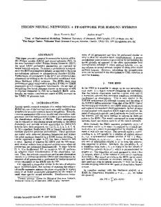
Example 2: Assume that we have to send the same data from pl to both p3 and p4 in figure I, the transfer may be represented by the message tree as shown in figure 3. Notice
il
"1
-
G&&6p4
0
e
n
2
6
Figure 3: Example of a message tree.
5 Algorithm overview Our synthesis algorithm is based on the genetic algorithm [SI which is an iterative and stochastic process that operates on a set of individuals (the population). Each individual represents a potential solution to the problem being solved, and is obtained by decoding the gene string of the individual. Initially, the population is randomly generated. Every individual in the population is assigned a fitness value which is a measure of its goodness with respect to the problem being considered. This value is the quantitative information the algorithm uses to guide the search for a feasible solution: The basic genetic algorithm consists of three major stages: selection, reproduction, and replacement. During the selection stage, a temporary population is created in which the fittest individuals have a higher number of instances than those less fit. A new population is then created by performing crossover followed by mutation. Finally, individuals of the original population is substituted by the newly created individuals in such a way that the most fit individuals are kept deleting the worst ones. A thorough description of genetic algorithms may be found in [41. There are two important issues which have to be addressed when formulating a problem to be solved by genetic algorithms; the encoding/decoding mechanism of the gene string of an individual, and the evaluation of thefimess of an individual.
that the data is first transferred to p z where it is stored in local memory. Then it is transfened independently from pz to p3 and p4, that is, p3 and p4 does not have to he ready at the same time. 0
prioaJeCc,is used as priority for message scheduling during fitness evaluation.
5.2
Fitness evaluation
The fitness value is calculated as a cost summation of four contributions, the higher the cost is, the less fit is the individual. The four contributions reflects p e r f o m c e , area, local memory usage, and huffer memory usage.
In order to be able to compare and tradeoff the different contributions, we define a cost normalization function, f&) where x is the difference between the value of the constraint and that of the implementation. Figure 4 gives an outline of fc(n). An x < 0 means violation of the corresponding con-
\
I""
5.1 Encoding/Decoding For a task graph containing IZ tasks and m dependencies, the corresponding gene string consist of n m genes, n task genes and m dependency genes. For each task zi its gene contains two integers, implg and prio.,. impl, identifies an implementation, i.e. an allocation. If a taskzi has ki possible implementations (as identified from its characterization), then the actual implementation is found as imply modulus ki. prio,( is a priority which is used when scheduling the task during the fitness evaluation. A dependency gene contains two integers, impldjgmcj and priodiJuccj,impld,,su, identifies a path between the processing elements on which q and its successors succ(zi) are dlocated. I.e. it identifies one of the possible paths in the architecture which is able to fulfill the communication represented by the data dependency impld,,,,, . This path is called a messuze tree. A message tree introduces a number of new tasks, &led communic&n tasks. These tasks reflects the communication as described in example 1, i.e. a write, a transfer, and a read task.
+
Figure 4: me cost normalization function. straint and a high cost is associated with this situation. The actual cost is determined by the slope a,.An n 2 0 means meeting the constraint. 6 determine how well this should be rewarded, in terms of a negative cost contribution, and the slope a2 how well even better implementations should be rewarded. Area
The simplest contribution is that of area, fc(Ao~-Aused)
CA = P@A
190
depends on which tasks are allocated on the corresponding processing element and on the functions used by these tasks. Le., the area used on processing element p j is expressed as,
selected is the one which has the earliest time point, fe, for its event, that being the starting or ending of its execution. This is determined as,
A,d
where the earliest time point for an event on a component ci is given as,
where fk denotes a function (as explained in section 2.2), and F ( y ) denotes all the functions used by zj. The first term is the area used by the tasks, whereas the second term is area used by the functions of the tasks, where each function is only implemented once.
if T~~is active tea(zj,ci)) otherwise
that is, if a task is already active on ci then the first event will be the ending of this task. If no task is currently active, the next event will be the earliest start time of the next task z j on ci, i.e. if ci is a processing element, then it is the first task in the priority queue of cj, else if ci is an interface, it is the first task of the FIFO queue. This task is found as the maximum end-time of all predecessors of 7.j and the end time of the last active task on ci.
Performance
Performance is calculated according to the deadline of the specification,
CT =
fc(tdeadline
- txhed)
The actual schedule, is found by performing a list based scheduling of the tasks on their allocated processing elements, and of the communication tasks on the corresponding interfaces and nets. List based scheduling relies on having a queue of ready tasks associated with each component. In our case we associate a p r i o r i 0 queue with each processing element and use the priority prioTjwhen inserting task zj into the queue. For interfaces, we use a FIFO quene as the way to prioritize communication tasks, as this is the usual way to implement an interface2. The scheduling algorithm for a single individual (i.e. solution) is as follows: 1. Decode the gene string to obtain an allocation of the tasks and message trees for the dependencies. The d e coding introduces a number of communicationtasks to be inserted in the task graph as outlined in example 2. In the following a task may be an original task or a communication task. 2. Find all tasks zi which are ready to be scheduled, that is, tasks which has no predecessors. These tasks are inserted into the priority queues of their respective components (found from implJ according to their priority (prioxi). 3. Find the next point in time, t , where something happens in the schedule, i.e. the starting or ending of a task q. If it is the end of a task, the end-point &(Ti) is set to t , and the successors of zi, for which all of their predecessors already have been scheduled, are inserted into theirrespectivequeues If it is the start of a task, the start-point tsaE(zi) is set to t. 4. If there are unscheduled tasks then goto step 3. Otherwise, the schedule is completed. Finding the next point in time where something happens, is the most complicated task of the scheduling algorithm, and will be explained in more details in the following. Let T~~ denote the last task on a component ci (i.e. a processing element or an interface), that is, the task currently active on ci or the last active task on ci. The next task to be awe are curreOt1y warking 0" supporfing other rypes Of inlafa-.
Local Memory
Local memory is calculated according to the peak memory usage, CM
=
f c ( M a v a i f ( P i ) -Mpepeak(Pi)) MEA
where the peak memory usage is calculated as described in example 1. Buffer Memory
Buffer memory is also calculated according to the peak memory usage, CB =
C fc(Bavaidii) - B p e d i r ) )
LEE*
where the peak buffer memory usage only has a dynamic contribution. This contribution is calculated in the same way as for the local memory.
6
Experimental Results
The presented algorithm is implemented in Java and is integrated within the LYCOS [lo] hardware/software. cosynthesis system. All experiments in this section are carried out on a 166MHz Pentium MMX mnning JDK1.1 under Linux, and execution times are given in seconds. The first experiment is that of figure 5 using a deadline of 400. Assume that we have an architecture corresponding to fignre 1, where the nets and interfaces are characterized as shown in table 1. In this experiment we assume that no task can execute on p1 and that the processors pZ,& and p4 each have a local memory of 1024 units of data. The task graph is first mapped to the architecture considering performance as the only cost. This results in a schedule, where zd is allocated on p2, TI and TI on p1. and TB and zg on p4. We get a solution with a schedule length of 323, which is much shorter than the 400 required, however,
191
~
PE
memory calculation shows, that p3 and p4 uses 22% and 29% more memory than available. If all constraints are considered we get a schedule, where $2 and $4 are allocated on pz, TI and ~3 on p3, and TS on p4. Here all memory constraints are met and the schedule length of 380 is within the deadline.
avai able static dynamic 5000 5000
p4
3262 3042
peak
1104 4366 761
3803
Table 2 Optimized memory usage for the tgff taskgmph that we handle the constraints of memory and huffer sizes which are typically found in embedded computer systems. We are currently working on extending our approach to handle conditionals and system-level pipelining, as well as handling several interface types. We are also wor!&g on including passive components such as global memory and display units. Finally, we are working on improving the execution time of the genetic algorithm. Acknowledgements
This work is supported by the Danish National Center for IT Research under grant no. CIT 149. fi
fz
I code I 210 I 180 I 190
I
code
I
210
I
240
I
200
References [I] A. Bender. Design of an Optimal Loosely Coupled Heterogeneous Multiprocessor System. In Eumpean Design and Test Conference, 1996. [Z] P. BjOmm-JOrgensen and J. Madsen. Critical Path Driven Cosynthesis for Heterogeneous T w e t Architectures. In 5th Intemationnl Worksho on HardwodSo am Codesi 15 - 19 1997. [3] R. Dick, D. L. R&es, and g % l y T G F F : ?ask Graphs for Free.In 6th International Workshopon Hordwaw3&are CodesigB Coded98 ages 97 - 101 1998. Genehc hlgorithm in Search, Oprimizntim & Ma[4] D. E. Go&=. chine Learnin . Addison-Wesle 1989. [SI E. S . H. Hou, Ansari, and H. gen. A Genetic Algorithm for Multiprocessor Scheduling. IEEE Tmnsaction on Poroilel and Distributed System, 5(2):113 - 120,1994. [6] J.-J. Hwang, Y.-C. chow, P. D. Anger, and C.-Y. Lee. Scheduling Precedence Graphs in Systems with Interpmcessor Communication Times. SIAM Journal of Computing 18(2):244-257 1989. [7] B. Keinhuis, E. Depretter, K. V ~ s e kand P. van de; Wolf. An Approach for Quantitative Analysis of Application-Specific DataAow Architectures. In l l t h In?. Conference ofAppUcatiom.spec@c Systems, Architectures and Processors pages 338 - 349 1997. , [8] K. Kuchcinski. Emkdded $stem Synthesis by Timng Constraints s$ving. .-"In loth Intemaional Symposium on System Synthesis, pages
Figure 5: Task graph and task characterization Interface
-
!*
fl. 13, I4,
is
paekage-size 16
trans. rate 1
32
1
16 32
8
fi.
Net nl
nz
6
8.
rnn-
_I*l
'77".
[lo] J. nhadsen, J. Grode. P. V. Knudsen, M. E. Petersen, and A. Haathausen. LYCOS: the Lyngby CO-SynthesisSystem. Design Automation orEmbeddedS stems, 2 2 195 235,,1997. [ I l l S . &hand A. ?Parker. S)%hesis of Aoplication-Specific Heterogeneous Multiprocessor Systems. Journal of Parollel and Dirnibuted Computin 16:338 - 351 1992. [12] S. M a s h and A. Parker. Syntliesa of Application-Specific Multiprocessor System Including Memory Components. Journal of VLSI SigmIPmcessing 8:97- 116 1994. [13] G. C. S h and E. I\. Lee. A C?ompile-Tme Scheduling Heuristic for Interconnection-Consvained Heterogeneous Processor Architectures. IEEE Transaction on Parallel and Dirtributed Systems. 4(2):175 187 1993. [I41 T. h n g and A. Gerasoulis. DSC: Scheduling parallel Tasks on an Unbounded Number of Processors. IEEE Tramaction on Paraileland Distributed System, 5(9):951- 967, 1994.
$8:
e.
192