1
Embedding of Large Boolean Functions for Reversible Logic
arXiv:1408.3586v1 [cs.OH] 15 Aug 2014
Mathias Soeken, Member, IEEE, Robert Wille, Member, IEEE, Oliver Keszocze, Student Member, IEEE, D. Michael Miller, Member, IEEE, Rolf Drechsler, Senior Member, IEEE
Abstract—Reversible logic represents the basis for many emerging technologies and has recently been intensively studied. However, most of the Boolean functions of practical interest are irreversible and must be embedded into a reversible function before they can be synthesized. Thus far, an optimal embedding is guaranteed only for small functions, whereas a significant overhead results when large functions are considered. In this paper, we study this issue. We prove that determining an optimal embedding is coNP-hard already for restricted cases. Then, we propose heuristic and exact methods for determining both the number of additional lines as well as a corresponding embedding. For the approaches we considered sums of products and binary decision diagrams as function representations. Experimental evaluations show the applicability of the approaches for large functions. Consequently, the reversible embedding of large functions is enabled as a precursor to subsequent synthesis.
I. I NTRODUCTION YNTHESIS of reversible circuits has been intensively studied in the recent past [4], [8], [9], [16], [19]. Since most Boolean functions of practical interest are irreversible, such functions are embedded into reversible ones prior to synthesis. Given an m-output irreversible function f on n variables, a reversible function g with m+k outputs is determined such that g agrees with f on the first m components. The overhead in terms of the k additional variables shall be kept as small as possible. The embedding is called optimal if k is minimal. Thus far, only synthesis approaches based on truth tables allow for a determination of an optimal embedding. However, determining an efficient embedding for large irreversible functions, i.e. functions with up to a hundred variables, is an open research problem which significantly hindered the development of scalable synthesis approaches for reversible logic. In this work, we study this issue from both, theoretical and practical, perspectives. First, we derive two lower bounds for determining the minimal value of k, namely (1) we show that already when m = 1 it is coNP-hard to determine if the minimal k equals n − 1 and (2) we show that, even when n − m is bounded by a constant, it is coNP-hard to decide if the minimal k equals n − m. Hence, computing the minimal
S
This work has been submitted to the IEEE for possible publication. Copyright may be transferred without notice, after which this version may no longer be accessible. M. Soeken, R. Wille, O. Keszocze, and R. Drechsler are with the University of Bremen, Germany, and the German Research Center for Artificial Intelligence (DFKI). D. M. Miller is with the University of Victoria, BC, Canada. M. Soeken is corresponding author:
[email protected]
number k of additional variables is not feasable in polynomial time unless P = NP. We then propose algorithms for both heuristic and optimal embeddings and evaluate for which cases an efficient application is possible. We differentiate between (1) determining the required number of additional lines and (2) determining the concrete embedding. The key element in both steps is to use sum-of-product expressions (SOPs) and binary decision diagrams (BDDs) which potentially allow for a more compact function representation compared to truth tables. As a result, an embedding methodology results which can process large irreversible functions for the first time. While so far efficient embedding of irreversible functionality was restricted to very small functions, the proposed approach enables embedding of functions containing hundreds of variables. We confirm this by comprehensive experimental evaluations. The contributions described in this paper are as follows: • We provide lower bounds for the embedding problem. • We present three algorithms for determining the number of additional lines of large irreversible functions, one heuristic algorithm (cube-based) and two exact ones (cube-based and BDD-based). • We propose two algorithms for embedding large irreversible functions, i.e. one exact algorithm (cube-based) and one heuristic algorithm (BDD-based) that respects the theoretical upper bound. • Finally, we provide open source implementations for all presented algorithms. The paper is organized as follows. Preliminary definitions are given in the next section. Section III provides the background on the synthesis of reversible function and motivates the problem that is addressed by this work. We present known upper bounds and derive new lower bounds for the problem in Section IV. Approaches for approximating and determining the minimal number of additional lines are described in Section V. Afterwards, approaches for exact and heuristic approaches are described in Section VI. Section VII presents and discusses the results from the experimental evaluation before the paper is concluded in Section VIII. II. P RELIMINARIES In this section we introduce notations. In Section II-A we introduce (reversible) Boolean functions, in Section II-B we review BDDs, and in Section II-C we define notations for SOPs.
2
x1 0 0 1 1
x2 0 1 0 1
y 0 0 0 1
γ1 0 0 1 0
γ2 0 1 0 0
κ 0 0 0 0 1 1 1 1
(a) Garbage outputs Fig. 1.
x1 0 0 1 1 0 0 1 1
x2 0 1 0 1 0 1 0 1
y 0 0 0 1 0 1 1 1
γ1 0 0 1 0 1 0 1 1
γ2 0 1 0 0 1 1 1 1
(b) Constant input
Embedding of the AND function
A. Boolean Functions and Reversible Boolean Functions def
Let IB = {0, 1} denote the Boolean values and let def
Bn,m = {f | f : IBn → IBm }
(1)
be the set of all Boolean functions with n inputs and m outdef puts, where m, n ≥ 1. We write Bn = Bn,1 for each n ≥ 1 and assume that each f ∈ Bn is represented by a propositional formula over the variables {x1 , . . . , xn }. Conversely, any m-tuple t of Boolean functions over variables {x1 , . . . , xn } corresponds to a unique Boolean function ft ∈ Bn,m . We assume that each function f ∈ Bn,m is represented as a tuple f = (f1 , . . . , fm ) where fi ∈ Bn for each i ∈ {1, . . . , m} and hence f (~x) = (f1 (~x), . . . , fm (~x)) for each ~x ∈ IBn . def Given a Boolean function f ∈ Bn,m the sets on(f ) = {~x ∈ def IBn | f (~x) 6= 0m } and off(f ) = {~x ∈ IBn | f (~x) = 0m } are called ON-set and OFF-set of f . It can easily be seen that on(f ) ∪ off(f ) = IBn . Assume f = (f1 , . . . , fm ) ∈ Bn,m and g = (g1 , . . . , gm′ ) ∈ Bn,m′ , where m′ ≥ m. We write f = g|m in case fi (~x) = gi (~x) for each ~x ∈ IBn and each i ∈ {1, . . . , m} and say that f is the m-projection of g. We say f ∈ Bn is valid if f (~x) = 1 for each ~x ∈ IBn . Given a function f = (f1 , . . . , fm ) ∈ Bn,m its characteristic function χf ∈ Bn+m is defined as ( 1 f (~x) = ~y def χf (~x, ~y) = (2) 0 otherwise for each ~x ∈ IBn and each ~y ∈ IBm . The characteristic function allows one to represent any multiple-output function as a single-output function. It can be computed from a multipleoutput function by adding to the variables {x1 , . . . , xn } the additional output variables {y1 , . . . , ym }: m ^
(yi ↔ fi (x1 , . . . , xn ))
(3)
i=1
Given a Boolean function f ∈ Bn over the variables X = {x1 , . . . , xn } and a variable xi ∈ X, we define the positive co-factor fxi ∈ Bn−1 and the negative co-factor fx¯i ∈ Bn−1 as fxi = f (x1 , . . . , xi−1 , 1, xi+1 , . . . , xn ) and fx¯i = f (x1 , . . . , xi−1 , 0, xi+1 , . . . , xn ), respectively. A function f ∈ Bn,m is called reversible if f is bijective, otherwise it is called irreversible. Clearly, if f is reversible,
then n = m. A function g ∈ Bn,m+k embeds f ∈ Bn,m , if g is injective and f ≡ g|m . The function g is called an embedding and the additional k outputs of g are referred to as garbage outputs and are denoted by ~γ later. We are interested in those embeddings of f , where k is minimal. Let def
µ(f ) = max{#f −1 ({~y }) | ~y ∈ IBm } denote the number of occurrences of the most frequent output def pattern. It is not hard to see that ℓ(f ) = ⌈log2 µ(f )⌉ is both an upper and a lower bound (and thus an optimal bound) for k. Thus, if k = ℓ(f ), then the embedding g is called optimal. Example 1: The AND function ∧ ∈ B2 can be embedded into a reversible function g ∈ B2,3 which is illustrated in Fig. 1a. The most frequent output pattern is 0, hence µ = 3. The embedding g is optimal. In order to obtain a reversible function for an embedding g, additional input variables might need to be added. Bijectivity can readily be achieved, e.g. by adding additional inputs such that f evaluates to its original values in case these inputs are assigned the constant value 0 and each output pattern that is not in the image of g is arbitrary distributed among the new input patterns. The additional inputs are referred to as constant inputs. Example 2: A constant input assignment, denoted κ, for the embedded AND function in Fig. 1a is given in Fig. 1b. Different algorithms that perform an optimal embedding of irreversible functions based on their truth table description have been proposed in the past [11]. B. Binary Decision Diagrams Binary Decision Diagrams (BDD) [3] are an established data structure for representing Boolean functions. While the general concepts are briefly outlined in this section, the reader is referred to the literature for a comprehensive overview [3], [7]. Let X = {x1 , . . . , xn } be a set of variables of a Boolean function f ∈ Bn . A BDD representing the function f is a directed acyclic graph F with non-terminal vertices N and terminal vertices T ⊆ { ⊥ , ⊤ } where N ∩ T = ∅ and T 6= ∅. Each non-terminal vertex v ∈ N is labeled by a variable from X and has exactly two children, low v and high v. The directed edges to these children are called low-edge and highedge and are drawn dashed and solid, respectively. A nonterminal vertex v labeled xi represents a function denoted σ(v) given by the Shannon decomposition [15] σ(v) = x¯i σ(low v) + xi σ(high v)
(4)
where σ(low v) and σ(high v) are the functions represented by the children of v with σ( ⊥ ) ≡ 0 and σ( ⊤ ) ≡ 1. The BDD F has a single start vertex s with σ(s) ≡ f . A BDD is ordered if the variables of the vertices on every path from the start vertex to a terminal vertex adhere to a specific ordering. Not all of the variables need to appear on a particular path and a variable can appear at most once on any path. A BDD is reduced if there are no two non-terminal vertices representing the same function, hence the representation of common subfunctions is shared. Complemented edges can
3
x1 1 0 1 − 1 1 Fig. 2.
x2 − 0 1 1 0 1
x3 − − − 0 − −
x4 0 − − − 1 1
x5 − − 1 − − 0
y1 1 0 0 0 1 1
y2 0 1 0 0 0 0
y3 0 0 1 1 1 1
Conversely, we can represent f also as a function that maps each cube from C to those output functions that are constructed from this cube. More formally, f is represented by a function Pf : C → P({f1 , . . . , fm })
(10)
where P denotes the power set and with
PLA representation
Pf (c) = {fi | c ∈ Ci }. additionally reduce the size of a BDD and are marked using a solid dot. In the following only reduced, ordered BDDs are considered and for brevity referred to as BDDs. Multiple-output functions can be represented by a single BDD that has more than one start vertex. Common subfunctions that can be shared among the functions decrease the overall size of the BDD. In fact, many practical Boolean functions can efficiently be represented using BDDs and efficient manipulations and evaluations are possible [3].
We refer to Pf as the PLA representation of f . Since the power set of all output functions is being used in several def places, we will use P(f ) = P({f1 , . . . , fm }) in the remainder for a more compact representation. We will later see that the PLA representation of a function turns out to be convenient to formulate algorithms. Example 3: The PLA representation of the function f = (f1 , f2 , f3 ) ∈ B5,3 with y1 = x1 x ¯4 ∨ x1 x¯2 x4 ∨ x1 x2 x4 x ¯5 , y2 = x ¯1 x ¯2 , y3 = x1 x2 x5 ∨ x2 x ¯3 ∨ x1 x ¯2 x4 ∨ x1 x2 x4 x¯5 .
C. Sum-Of-Product Representation Each Boolean function f ∈ Bn can be represented in SumOf-Product (SOP) representation in which f is of the form f (x1 , . . . , xn ) =
k _
p p x1i,1 x2i,2
· · · xpni,n
(5)
i=1
with polarities pi,j ∈ {0, 1, 2} ¯ x xp = x 1
for j ∈ {1, . . . , n} and if p = 0, if p = 1, if p = 2.
(6)
If p 6= 2, xp is called a literal, otherwise xp is referred to p p p as don’t care. We call each ci = x1i,1 x2i,2 · · · xni,n a cube1 of weight ω(ci ) = #{j | pi,j 6= 2}. (7) That is, the weight refers to the number of literals in ci . Note that # on(ci ) = 2n−ω(ci ) , i.e. by removing one literal one doubles the number of input assignments that satisfy ci . The set (8) dc(c) = {xpi i | i ∈ {1, . . . , n}, pi = 2} refers to all variables that are don’t care and hence not contained as literal in the cube. One can also represent f by its cubes {c1 , . . . , ck } and we write f ⊸ {c1 , . . . , ck }
(9)
where ⊸ reads “is constructed of.” A multiple output function f = (f1 , . . . , fm ) ∈ Bn,m is represented by m such sum-of-product forms, i.e. fi ⊸ Ci for i ∈ {1, . . . , m} where each Ci is a set of cubes. All cubes of f are then given by C=
m [
Ci .
i=1 1 Often,
also the term monom is used synonymously.
is illustrated by the table in Fig. 2. As before, we make use of the convention yi = fi (x1 , . . . , x5 ). Each input cube of f is represented by its polarities with the exception that we write − instead of 2. For each output function we write 1, if the corresponding cube is in its constructing set, otherwise 0. The table shall not be confused with a truth table, in particular the 0’s in the output columns do not indicate that the functions evaluate to 0 for the corresponding input cube. As an example, we have f1 (x1 , x2 , x ¯3 , x4 , x ¯5 ) = 1 due to the sixth cube. However, this input pattern is also contained in the fourth cube which is not in the constructing set of f1 . III. S YNTHESIS
OF
R EVERSIBLE F UNCTIONS
Reversible circuits on r lines composed of special reversible gates, e.g. Toffoli gates, represent reversible functions of r variables. In turn, every reversible function can be realized with a reversible circuit. The problem of finding a reversible circuit for a given function is called synthesis and, since most of the functions of practical interest are irreversible, we are considering the following synthesis problem in this paper: Given an arbitrary Boolean function f ∈ Bn,m , a reversible circuit should be determined that represents g ∈ Br,r such that g embeds f . The synthesis of reversible functions has been an intensively studied research area in the last decade. Initially, algorithms based on truth table representations have been proposed [5], [9]. Due to their non-scalable representation, none of these is capable of efficiently synthesizing functions with more than 20 variables. This fact is reflected in the first two rows in Table I. The R in the respective rows denotes that these approaches are only directly applicable for reversible functions. However, irreversible functions are handled by embedding them first as described in the previous section. Moreover, an
4
TABLE I S YNTHESIS OF REVERSIBLE FUNCTIONS Representation S Scalability E Overhead Truth table (exact) R ≤ 7 variables y minimal Truth table (heuristic) R ≤ 20 variables y minimal Symbolic I ≈ 100 variables N/A large Symbolic (QMDDs) R ≈ 100 variables n minimal S: Supports reversible (R) or also irreversible (I) functions E: Embedding approaches are available (y) or not (n)
optimal embedding and therefore a minimal overhead in terms of additional variables can be guaranteed since the value of ℓ(f ) can readily be determined from the truth table, in other words r = m + ℓ(f ). In order to synthesize larger functions, researchers have been investigating the use of symbolic representations. An approach based on BDDs [20] is one of the first solutions able to synthesize functions with more than one hundred variables (as summarized in the third row of Table I). In particular, by using BDDs it is also possible to directly start with the irreversible function representation as the embedded takes place implicitly during synthesis (denoted by I in the second column of Table I). However, the newly achieved scalability is traded off against a large number of additional variables which is much larger than the upper bound [21], in other words r ≫ m + n. The large number of additional variables results from the fact that this algorithm performs synthesis in a hierarchical fashion rather than considering the function as a whole. Determining an optimal embedding similar to the truth tablebased approaches is not applicable. Although optimization approaches exist that reduce additional variables in a postsynthesis step [22], a satisfying result can rarely be achieved as evaluated in [21]. Following these considerations, an alternative has been proposed in [19] that exploits another symbolic representation and relies on reversible functions. For this purpose, Quantum Multiple-values Decision Diagrams QMDDs [10] are utilized which are data-structures particularly suited for the representation of reversible functions. For the first time, this enabled the synthesis of reversible functions with up to 100 variables and without adding any additional variables. However, this algorithm is of not much help, since so far it was unknown how to embed the given irreversible function into a QMDD representing the reversible embedding (as summarized in the forth row of Table I). In summary, synthesis of reversible circuits for irreversible functions always requires an efficient embedding. For small functions, this is no problem and in fact, optimal embeddings can readily be obtained. In contrast, if larger functions are addressed, previous solutions led to significantly high overhead. Although scalable synthesis methods for large reversible functions are available, how to derive the respective embeddings is unknown so far. In this paper, we are addressing this issue by lifting embedding from truth table based approaches to symbolic ones. For this purpose, we are exploiting observations by Bennett on upper bounds and general embeddings. Additionally, we
use the symbolic representation of BDDs. However, we first consider the theoretical complexity of the embedding problem. IV. B OUNDS
FOR THE
N UMBER
OF
A DDITIONAL L INES
A. Upper Bound An upper bound for the number of lines can easily be determined as described by the following proposition. Proposition 1: Given a function f ∈ Bn,m . Then at most ℓ(f ) = n additional lines are required to embed f . Proof: The value of µ(f ) is maximized if there exists one ~y ∈ IBm such that for all ~x ∈ IBn we have f (~x) = ~y . In this case µ(f ) = 2n . Hence, ℓ(f ) = ⌈log2 2n ⌉ = n B. Lower Bounds In this section, we concern ourselves with the following question: Given a Boolean function f ∈ Bn,m and some ℓ ≥ 0, does ℓ = ℓ(f ) hold? We prove two coNP lower bounds in this section, one even when m is a fixed and one even when ℓ is fixed. It is clear that we cannot hope for an efficient procedure for computing an optimal embedding for a given f ∈ Bn,m if we cannot even compute ℓ(f ) efficiently. Proposition 2: For every fixed m ≥ 1 it is coNP-hard to decide, given f ∈ Bn,m with n ≥ m, whether ℓ(f ) = n − m. Proof: We give a polynomial time many-one reduction from the validity problem, i.e. to decide for a given propositional formula whether it is valid, a coNP-complete problem. Let ϕ be a propositional formula over the variables def {x1 , . . . , xj }. We put n = j + m. We will compute in polynomial time an m-tuple t = (ψ1 , . . . , ψm ) of propositional formulas over the variables {x1 , . . . , xj+m } such that ϕ is valid if, and only if, ℓ(ft ) = n − m = j. We put ψi (x1 , . . . , xj+m )
def
=
xj+i ∧ ϕ(x1 , . . . , xj )
(11)
for each i ∈ {1, . . . , m}. The correctness of the reduction follows immediately from the following equivalences: ϕ is valid ⇔
#{~x ∈ IBj | ϕ(~x) = 1} = 2j
(11)
⇔
∀~y ∈ ft (IBj+m ) : #{~x ∈ IBj+m | ft (~x) = ~y } =
⇔ ⇔
µ(ft ) = 2j ℓ(ft ) = j = n − m
2j+m 2m
Looking at the proof of Proposition 2 we note that we required ℓ to be part of the input for the lower bound to work since we fixed m. Moreover the lower bound already holds when m = 1 and thus when ℓ = n − 1. The dual question arises whether a lower bound can be proven when ℓ is a fixed constant. Indeed, we prove that computing ℓ(f ) is already coNP-hard for every fixed ℓ ≥ 0 (i.e. the input to the problem only consists of f and the value ℓ is treated as a fixed constant). Proposition 3: For each fixed ℓ ≥ 0 it is coNP-hard to decide for a given f ∈ Bn,m whether ℓ(f ) = ℓ.
5
Proof: We give a polynomial time many-one reduction from the validity problem for propositional formulas. For simplicity we only give the proof for ℓ = 0. The case ℓ > 0 works completely analogously. Fix a propositional formula ϕ ∈ Bn over the variables {x1 , . . . xn }. We will compute in polynomial time a function f = (f1 , . . . , fn ), where each fi is presented by a propositional formula ϕi over the variables {x1 , . . . , xn } such that ϕ is valid if, and only if, f is injective. We set def
ϕi (x1 , . . . , xn ) = xi ∧ ϕ(x1 , . . . , xn ) ∧ ϕ(0, . . . , 0)
(12)
for each i ∈ {1, . . . , n}. For correctness, we have to show that ϕ is valid if, and only if, ℓ(f ) = 0, which in turn is equivalent to f being injective. Let us first assume that ϕ is valid. Then ϕi is logically equivalent to xi for each i ∈ {1, . . . , n} by definition (12). def Thus, f is equivalent to the identity idn ∈ Bn,n , i.e. idn (~x) = n ~x for each ~x ∈ IB . Conversely, assume that ϕ is not valid. Then there exists some ~x ∈ IBn with ϕ(~x) = 0. We make a case distinction. In case ~x = 0n , we immediately have that ϕi is logically equivalent to 0 and thus f is not injective. Now assume that ~x 6= 0n . Since ϕ(0n ) = 0n and ϕ(~x) = 0n and also ~x 6= 0n , the function f is not injective. We note that two simple lower bound corollaries follow from Proposition 2 and 3: (1) it is coNP-hard to decide if for a given function f ∈ Bn,n and a given ℓ ≥ 0 whether there exists an injective g ∈ Bn,n+ℓ that embeds f , (2) there exists no polynomial time algorithm that computes, given a function f ∈ Bn,n , the minimal ℓ ≥ 0 such that f can be embedded by some function g ∈ Bn,n+ℓ unless P = NP. V. D ETERMINING
THE
N UMBER
OF
A DDITIONAL L INES
In this section we propose three algorithms to determine the number of additional lines. The first algorithm approximates the number of lines while the second and third one determine the minimal number. A. Heuristic Cube-based Approach The first approach approximates the number of cubes and is based on the PLA representation of a multiple output function. The approach is an extension of an algorithm presented in [21]2 . Given a function, one can approximate the minimal number of additional variables that are needed to embed the function using the following algorithm. Algorithm H (Heuristic Cube-based Approach). This algorithm approximates µ(f ) by µ ˆ(f ) for a given function f ∈ Bn,m given in PLA representation Pf : C 7→ P(f ). An auxiliary array MU[o] for o ∈ P(f ) is used to compute possible candidates for µ ˆ(f ). H1. [Initialize.] Set MU[o] ← 0 for each o ∈ P(f ). H2. [Loop over C and update MU.] For each c ∈ C, set MU[Pf (c)] ← MU[Pf (c)] + # on(c). 2 In [21], the algorithm does not consider the OFF-set of the function and, hence, may return an under approximation.
x1 1 0 1 − 1 1 Fig. 3.
x2 − 0 1 1 0 1
x3 − − − 0 − −
x4 0 − − − 1 1
x5 − − 1 − − 0
y1 1 0 0 0 1 1
y2 0 1 0 0 0 0
y3 0 0 1 1 1 1
8 8 4 8 4 2
12 6
PLA representation of a Boolean function
H3. [Count off(f ) in MU.] Set MU[∅] ← # off(f ). H4. [Determine µ ˆ(f ).] Set µ ˆ(f ) ← max{MU[o] | o ∈ P(f )}. Remark 1: Although the set P(f ) is exponentially large, Algorithm H can be efficiently implemented, since it only needs to consider those elements that are in the image of Pf . Step 3 can be implemented using BDDs. Example 4: Consider the function given in Fig. 3. Algorithm H basically assigns the number of input patterns that are represented by an input cube to each line of the PLA representation. In order to approximate, we assume that the 0s in the table are part of the output pattern. Values of lines with the same output pattern are added. The OFF-set of the function is not mentioned in the table representation and can be described by the cube 011-- that corresponds to 4 input pattern. The algorithm computes, that approximately 4+8 = 12 input patterns map to the output pattern 001 which corresponds to the computed approximation for µ(f ) obtained from Algorithm H. Hence, 3 + ⌈log2 12⌉ = 7 lines may be sufficient to realize this function as a reversible circuit. The determined value for µ ˆ(f ) is still an approximation, since overlaps of the input cubes are not yet considered. For example, the two input cubes discussed in Example 4 share some equal input patterns, i.e. the determined number of 12 occurrences for the output pattern 001 is an approximation. In fact the output patterns that are assumed for the approximation may have nothing in common with the real output patterns of the function that is described by the PLA representation. Consequently, µ ˆ(f ) can be smaller than µ(f ). An example for this case is given in the following section. However, the results from the experimental evaluation presented in Section VII will show that the approximation is often close to the exact value. B. Exact Cube-based Approach If we had a PLA representation Pf′ : C ′ → P(f ) in which no input cube overlaps, i.e. on(ci ) ∩ on(cj ) = ∅ for all pairwise ci , cj ∈ C ′ , one can guarantee that µ ˆ(f ) = µ(f ) after applying Algorithm H to Pf′ . The expressions represented by such PLAs are called disjoint sum-of-products (DSOP) in the literature and several algorithms to derive such a representation have been described in the past. The most recent results can be found e.g. in [2], [14]. We create a DSOP representation based on an algorithm described in [21] that particularly addresses multiple-output functions. Please note that the compact representation of a PLA representation highly depends on overlapping input cubes. As
6
Pf′ ← Pf′ ∪ {(c ∧ c′ , o ∪ o′ )} Pf′ ← Pf′ ∪ {(c′ ∧ c¯, o′ )}
Pf ← Pf ∪ {(c ∧ c¯′ , o)}
c ∧ c¯′
c ∧ c′
c′ ∧ c¯
0 1 1 1
0 1 1 0 1
0 -
Pf - - 1 - 1 1 0
0 0 0 1 1
1 0 0 0 0
Pf′ 0 ◮ 1 - - 0 - 1 0 0 1 1 1 1
(a) Moving first cube e = (c, o) Fig. 4.
e′ = (c′ , o′ ) 1 1 1
Illustration for step 3 in Algorithm D
a result, the PLA representation of the DSOP expression is possibly very large. In the worst case, the whole truth table is reconstructed. Algorithm D (Disjoint Sum-of-Product Computation). Given a PLA representation Pf : C → P(f ) of a function f ∈ Bn,m , this algorithm computes a new PLA representation Pf′ : C ′ → P(f ) where no input cubes overlap, i.e. on(ci ) ∩ on(cj ) = ∅ for all pairwise different ci , cj ∈ C ′ . In the algorithm, Pf and Pf′ are treated as mutable relations. D1. [Terminate?] If Pf = ∅, terminate. D2. [Pick an entry from Pf and iterate over Pf′ .] Pick and remove one entry e = (c, o) from Pf , i.e. set Pf ← Pf \ {e}. If there exists an overlapping cube e′ = (c′ , o′ ) ∈ Pf′ , i.e. c ∧ c′ 6= ⊥, perform step 3. If no such e′ exists, set Pf′ ← Pf′ ∪ {e} and return to step 1. D3. [Update Pf and Pf′ .] Remove the entry e′ from Pf′ , i.e. set Pf′ ← Pf′ \{e′ }. Keep one “remaining part” for Pf , i.e. Pf ← Pf ∪ {(c ∧ c¯′ , o)} and the other one for Pf′ , i.e. Pf′
←
Pf′
1 1 0 1
0 -
Pf - 1 - 1 1 0
0 0 1 1
0 0 0 0
Pf′ 1 1 - - 0 - 1 0 0 1 ◮ 0 0 - - - 0 1 0 1 1
(b) Moving second cube
◮ 1 1 1
1 1 0 1
0 -
Pf 1 1 - 1 1 0
0 0 1 1
0 0 0 0
1 ◮ 1 1 1 0 0 1 ◮ 1 0 1 ◮ 1 1 -
Pf′ 0 1 - 0 0 0
1 0 1 1
0 1 0 0
1 0 0 0
0 0 1 1 1 1 1 1 1 1 1 1
0 1 0 0 1 1 1 1 1 1 1 1
0 0 0 0 0 1 1 1 1
Pf′ - - 0 1 0 0 0 1 1 0 1 1 0 0 0 1 1 0 1 1
0 0 1 1 1 1 1 0 1 1 1 0
1 0 0 0 0 0 0 0 0 0 0 0
0 1 0 1 1 1 1 1 0 1 1 1
(d) PLA for DSOP expression
(c) Merging third cube Fig. 5.
DSOP computation for the function in Fig. 3
empty. Affected cubes in steps are marked by ‘◮’. Also the second cube can be moved without merging since it does not intersect the first one. The third cube to be moved from Pf to Pf′ has the input pattern c = x1 x2 x5 . It intersects with the current first cube in Pf′ which has the input pattern c′ = x1 x¯4 . The “remaining part” for Pf is ¯4 = x1 x2 x4 x5 . x1 x2 x5 ∧ x1 x Analogously we have x1 x2 x5 ∧ x1 x ¯4 = x1 x ¯2 x ¯4 ∨ x1 x2 x ¯4 x ¯5 which yields two new entries to be added to Pf′ . The current entry is updated by the intersection x1 x2 x5 ∧ x1 x¯4 = x1 x2 x ¯4 x5
′
′
∪ {(c ∧ c¯, o )}.
Pf′
Add the intersection to by combining the output sets, i.e. Pf′ ← Pf′ ∪ {(c ∧ c′ , o ∪ o′ )}. Algorithm D transforms the initial PLA representation Pf into the initial empty PLA representation Pf′ which represents the same function as DSOP expression. As long Pf is non-empty an entry e = (c, o) is chosen for which the following case distinction is applied. If c does not intersect with any other input cube in Pf′ , the entry e is removed from Pf and directly added to Pf′ . Otherwise, i.e. if there exists an entry e′ = (c′ , o′ ) with c ∧ c′ 6= ⊥, step 3 is performed. What happens in this step after e′ has been removed from Pf′ is best illustrated by means of Fig. 4. The ON-set of c ∨ c′ is partitioned into three parts. The part of c that does not intersect c′ remains in Pf , and analogously, the part of c′ that does not intersect c remains in Pf′ . The intersection is also added to Pf′ , however, the corresponding output functions are combined. Example 5: An example application of Algorithm D is demonstrated in Fig. 5 based on the PLA of Fig. 2. Clearly, the first cube can be moved without merging since Pf′ is initially
for which the corresponding output functions are merged. All other steps are not shown explicitly. The final PLA representation for Pf′ is given in Fig. 5(d). Correctness and completeness: We now prove that Algorithm D is sound and complete. Lemma 1: Algorithm D is complete. Proof: We show that the algorithm terminates for every input function f . For this purpose, we show that in every iteration the size of the ON-set of the function represented by Pf decreases. Consequently, we eventually have Pf = ∅ which leads to termination in step 1. We perform a case distinction on whether a cube e′ exists in step 2. If such a cube e′ does not exist, e = (c, o) is removed from Pf and we have c 6= ⊥. Further, nothing is added to Pf in this case. Otherwise, first c is removed from the input cubes and afterwards c∧¯ c′ is added. However, since by assumption c∧c′ 6= ⊥, we have # on(c ∧ c¯′ ) < # on(c). Lemma 2: Algorithm D is sound. Proof: Clearly, Pf′ does not contain overlapping input cubes due to step 3. We now show that in step 1 the function represented by Pf ∪ Pf′ equals f . Since eventually Pf = ∅,
7
0 0 1 1 1 1 1 1 1 1 Fig. 6.
0 1 0 0 1 1 1 1 1 1
0 0 0 1 1 1
Pf′ - - 0 1 1 1 0 1 0 0 0 0 1 1 0
0 0 1 1 0 1 1 1 1 1
1 0 0 0 0 0 0 0 0 0
overlapping input cubes:
0 1 0 1 1 1 1 0 1 1
0 1- 1 - 0 10 0 0- 1 - 0 11 1 - - - - 0 11 For this PLA representation Algorithm H will compute the following output pattern occurrences: 000 7→ 8
PLA representation after post compaction
Pf′ represents f . We perform a case distinction on whether a cube e′ exists in step 2. If such a cube e′ does not exist, the case is trivial, since e is removed from Pf and directly added to Pf′ . For the case that a cube e′ does exist one can readily observe based on the partition in Fig. 4 that the ON-set of Pf ∪Pf′ does not change. Since the output functions are combined for the intersection c∧ c′ , also the functional semantics of f is preserved. Post compaction: It is possible to compact the resulting PLA representation that is returned by Algorithm D. For this purpose we create a BDD for each occurring output pattern from the input cubes. This step is only sound because the input cubes do not overlap. By traversing all paths in the BDD we can obtain a new PLA representation for each output cube. It turns out that the PLA representation for the input cubes is more compact compared to the one that resulted from applying Algorithm D. Example 6: The application of Algorithm D in Example 5 yields a PLA representation that consists of 12 cubes. Applying post compaction as post process yields a PLA representation that consists of 10 cubes (cf. Fig. 6). In the experimental evaluation we will demonstrate that much higher compression can be achieved with this method. An under approximating example: As discussed in Section V-A, Algorithm H can yield an under-approximation for µ(f ). Consider the following PLA representation for a function with 5 input variables, 3 output variables, and 6 monoms: 0 0 - 1 - 0 01 0 0 01 0 0 01 1 1 11 - 0 01 - - - 1 - 0 10 1 - - - 1 0 11 1 - - - 0 0 11 Algorithm H will compute the following output pattern occurrences: 000 7→ 8
001 7→ 7
010 7→ 16
011 7→ 16
Note that the sum of all occurrences is 47 although the function only has 32 output patterns. Algorithm H yields µ ˆ(f ) = 16 which corresponds to 4 additional output variables and therefore a total of 7 variables in a reversible embedding. After applying Algorithm D (together with post compaction) one obtains the following equal PLA representation with no
010 7→ 4
011 7→ 20
Since the PLA is representing a DSOP expression we have µ ˆ(f ) = µ(f ) = 20 which corresponds to 5 additional output variables and a total of 8 variables in a reversible embedding. C. BDD-based Approach All approaches presented thus far use a PLA representation in computing or approximating µ(f ). However, sometimes such a representation is not available but the functions that are being considered can be represented as BDDs. In this section an algorithm is described that computes µ(f ) directly on the BDD representation of an irreversible function f ∈ Bn,m in memory with f (x1 , . . . , xn ) = (y1 , . . . , ym ). For this purpose, first the characteristic function χf is computed as described in (2). For this purpose, the BDD of the characteristic function is constructed assuming the variable order x1 < · · · < xn < y1 < · · · < ym . Then, let Vx be the set of all vertices that are labeled xi for some i and whose immediate parent is labeled yj for some j. The on-sets of the functions represented by each vertex in Vx form a partition of all 2n input patterns. This can be exploited by using the following proposition. Proposition 4: In the BDD of χf every path from the start vertex to a vertex in Vx visits all variables y1 , . . . , ym . Further, each vertex in Vx has only one incoming edge. Proof: Assume that there is a path from the start vertex to a vertex v in Vx in which a variable vj is not visited. Then, the monom represented by v maps to more than one output in f which contradicts that f is a function. The same argument holds when we assume that v has more than one incoming edge. Now µ(f ) can easily be computed using the vertices in Vx , i.e.: µ(f ) = max{# on(σ(v)) | v ∈ Vx } (13) Example 7: The BDD for the characteristic function of the example in Fig. 3 is given in Fig. 7. Vertices from the set Vx are filled in gray and annotated by the output pattern they are mapping to. Based on the paths one can count the minterms of each node which results in: 100 7→ 4 101 7→ 9 010 7→ 8 001 7→ 6
000 7→ 5
The numbers coincide with the results from Example 5. VI. E MBEDDING I RREVERSIBLE F UNCTIONS In this section, we describe two approaches that construct a reversible embedding for a given irreversible function f . The first approach takes f as a DSOP expression and guarantees a minimal number of additional lines. The second approach takes f as a binary decision diagram and is heuristic.
8
f
Algorithm E (Cube-based Embedding). Given a function f ∈ Bn,m represented as a DSOP, this algorithm generates a partial reversible function g ∈ Br,r with
y1 y2
y2
y3 100
y3
x1
x1
x2
x2
x3 x4
g(κ1 , . . . , κp , x1 , . . . , xn ) = (y1 , . . . , ym , γ1 , . . . , γℓ(f ) )
101
y3 x1
x2
010 001
x2
x3 x4
x4
x1
x1 x2
000
x2
x3 x4
κ1 < y1 < κ2 < y2 < · · · < xn < γℓ(f ) ,
x5 ⊤ Fig. 7.
BDD for the characteristic function of the example in Fig. 3
A. Exact Cube-based Approach First, we will describe an exact embedding approach with respect to the number of additional lines that makes use of Algorithms H and D from the previous section. Given an irreversible function represented as a PLA, it is first transformed to represent a DSOP expression to determine the optimal number of additional lines. Then a reversible function is created by traversing all cubes of the DSOP expression. The algorithm requires the function to be represented as a DSOP expression in order to guarantee that no two input cubes have a non-empty intersection. Also, the algorithm creates a partial reversible function, i.e. not for all input patterns an output pattern is specified. However, all specified patterns in the reversible function are fully specified, i.e. they have no don’t-care values. We are making use of two helper functions in the following algorithm which are defined as follows. Given a function f ∈ Bn,m and a set of output functions o ∈ P(f ), the function ( m ^ yi if fi ∈ o, def cube(o) = y¯i otherwise, i=1 creates a cube that contains a positive literal yi if the function fi is contained in o and a negative literal y¯i otherwise. Given a set of variables x1 , . . . , xn the function inc(x1 , . . . , xn ) = (s1 , . . . , sn ) computes the increment of the integer representation given by xn xn−1 . . . x1 , i.e. def
si = xi ⊕
i−1 ^
and r = p + n = m + ℓ(f ) that embeds f and is represented as its characteristic χg function using a BDD. Let Pf = {(c1 , o1 ), . . . , (ck , ok )} be the PLA representation for the DSOP expression of f , i.e. no input cubes overlap. E1. [Initialization.] Let χg ← ⊥ be a BDD with variable ordering
xj
for i ∈ {1, . . . , n}.
j=1
Note that both functions, cube and inc, are easy to implement using BDD manipulation. We are now ready to formulate the algorithm to embed a truth table based on a function’s PLA representation.
i.e. inputs and outputs of χg appear in alternating order. Set ℓ ← ℓ(f ) where ℓ(f ) = ⌈log2 µ(f )⌉ is obtained from Algorithm H. Further, set j ← 0 and CNT[o] ← 0 for o ∈ P(f ). E2. [Loop over C.] If j = k, terminate. Otherwise, set j ← j + 1, c ← cj , and o ← oj . E3. [Add cube to χg .] Let (s1 , . . . , sℓ ) = incq (γ1 , . . . , γℓ ) where q = CNT[o], i.e., inc is applied q times to the garbage outputs γ1 , . . . , γℓ and the values are stored in s1 , . . . , sℓ . Also, let {d1 , . . . , dt } = dc(c)
with d1 < d2 < · · · < dt
be the indexes of variables which are set don’t-care in the input cube c. Let e = |{z} c ∧ cube(o) ∧ | {z } x’s
y’s
p ^
κ ¯i ∧
t ^
i=1
i=1
| {z }
|
κ’s
(xdi ↔ si ) ∧
ℓ ^
s¯i
i=t+1
{z
γ’s
}
(14) and set χg ← χg ∨ e. Also, set CNT[o] ← CNT[o] + # on(c). Return to step 2. In step 1, an empty BDD χg is created that interleaves inputs and outputs in its variable ordering. The size of the BDD is determined by calculating the minimal number of additional lines ℓ(f ) using Algorithm H after applying Algorithm D. The auxiliary array CNT is used to store how often an output pattern o has been used and is initially initialized to 0. Step 2 manages the algorithm’s loop over step 3. In each iteration one entry of Pf is added to g. Step 3 creates a cube e in (14) for the characteristic function χg based on the entry (c, o) of the PLA representation Pf . This cube e contains all required “ingredients,” i.e. values for x’s, y’s, κ’s, and γ’s referring to inputs, outputs, constants, and garbage outputs, respectively. • Input assignments for x1 , . . . , xn are directly obtained from the input cube c. • Output assignments for y1 , . . . , ym are obtained from cube(o). • Constants κ1 , . . . , κp are all assigned 0. • The idea is to relate the values of the don’t-care variables of c to the garbage outputs γ1 , . . . , γℓ . Since there may
9
be equal output patterns, an offset q = CNT[o] is taken into account. To calculate the offset, the ‘inc’ function is applied to the γ variables q times. If there are less don’t-care variables than garbage outputs, the remaining s variables are inverted. Since ℓ is also obtained based on the number of don’t-care variables in c, there are never more don’t-care variables than garbage outputs in this step, i.e. t ≤ ℓ. Example 8: We apply Algorithm E to the function with the PLA representation 0 1- 1 - 0 1 0 0 0- 1 - 0 1 1 1 - - - - 0 1 1 Fig. 8.
that has already been used in Section V-B. Initially we set χg ← ⊥. Also we assign CNT[{f2}] ← 0 for the first pattern and CNT[{f2, f3 }] ← 0 for the second and third pattern. Since µ(f ) = 20 we have ℓ(f ) = 5 and therefore the reversible function g ∈ B8,8 maps inputs (κ1 , κ2 , κ3 , x1 , x2 , x3 , x4 , x5 ) to outputs (y1 , y2 , y3 , γ1 , γ2 , γ3 , γ4 , γ5 ). For the first cube we have (s1 , . . . , s5 ) = (γ1 , . . . , γ5 ) and hence we have e1 = κ ¯1κ ¯2κ ¯3 x ¯1 x2 x4 y¯1 y2 y¯3 (x3 ↔ γ1 )(x5 ↔ γ2 )¯ γ3 γ¯4 γ¯5 and we set CNT[{f2}] ← 4. For the second cube we also have (s1 , . . . , s5 ) = (γ1 , . . . , γ5 ) and hence we have e2 = κ ¯1κ ¯2κ ¯3 x ¯1 x ¯2 x4 y¯1 y2 y3 (x3 ↔ γ1 )(x5 ↔ γ2 )¯ γ3 γ¯4 γ¯5 and we set CNT[{f2, f3 }] ← 4. For the third cube we have (s1 , . . . , s5 ) = inc4 (γ1 , . . . , γ5 ), i.e. s1 s2
= =
γ1 γ2
s3 s4
= =
γ3 ⊕ 1 γ4 ⊕ γ3
s5
=
γ5 ⊕ γ3 γ4 .
Hence, we have e3
(x4 ↔ γ¯3 )(x5 ↔ (γ4 ⊕ γ3 ))(¯ γ5 ⊕ γ3 γ4 )
and update CNT[{f2, f3 }] ← 20. Overall, the partial reversible function embedding f is given by χg = e1 ∨ e2 ∨ e3 . Correctness and completeness: Since the only loop in Algorithm E is bound by the number of cubes in the PLA representation, completeness is readily shown and it is left to show soundness. Lemma 3: Algorithm E is sound. Proof: To proof soundness we show that (i) the input patterns are unique, (ii) the output patterns are unique, and (iii) g embeds f . Since the PLA represents a DSOP expression for f , it does not contain overlapping input cubes, and (i) holds trivially. Also (iii) follows immediately from (14). Only (ii) requires
x1 . . . xn 0...0 .. .
y1 . . . ym f1 (~x) . . . fm (~x) .. .
γ1 . . . γn 0...0 .. .
0 . . . 00 0 . . . 01 .. .
1...1 0...0 .. .
f1 (~x) . . . fm (~x) f1 (~x) . . . fm (~x) .. .
1...1 0...0 .. .
0 . . . 01 .. .
1...1 .. .
f1 (~x) . . . fm (~x) .. .
1...1 .. .
1 . . . 11 .. .
0...0 .. .
f1 (~x) . . . fm (~x) .. .
0...0 .. .
1 . . . 11
1...1
f1 (~x) . . . fm (~x)
1...1
Bennett embedding scheme
some more thorough argument. We already motivated above that t ≤ ℓ in step 3. Also since ℓ is obtained from Algorithm H, one can see that CNT[o] ≤ MU[o] is invariant. And since further ℓ ≤ log2 MU[o], the assigned value for the garbage lines cannot “overlap.” B. Heuristic BDD-based Embedding In this section, an approach is presented that embeds a function directly using BDDs. That is, the possibly costly way of having an PLA representation is omitted by directly starting from BDDs. These BDDs must be stored in memory and may have been created by any algorithm. For this purpose, the idea of embedding as proposed by Bennett [1] who has initially proven the upper bound from Proposition 1 is adapted. In his constructive proof he already applied an explicit embedding which is known as Bennett Embedding and given as follows: Theorem 1 (Bennett Embedding): Each function f ∈ Bn,m is embedded by the function g ∈ Bm+n,m+n such that def
g(κ1 , . . . , κm , x1 , . . . , xn ) = (y1 , . . . , ym , γ1 , . . . , γn ) (15) with yi (κ1 , . . . , κm , x1 , . . . , xn ) = κi ⊕ fi (x1 , . . . , xn )
= κ ¯1κ ¯2κ ¯3 x1 y¯1 y2 y3 (x2 ↔ γ1 )(x3 ↔ γ2 ) ∧
c1 . . . cm 0 . . . 00 .. .
(16)
and γi (κ1 , . . . , κm , x1 , . . . , xn ) = xi .
(17)
Proof: The embedding is illustrated in Fig. 8. Assume g is not injective, hence there is an output pattern that occurs at least twice. In particular, the function values for γi must equal and according to (17) also the respective assignments for inputs xi must equal. But if the assignments for the inputs xi are the same, then the assignments for the inputs κj must differ and due to (16) also the function values for yi , contradicting our assumption. Conducting the embedding posed by Theorem 1 on a truth table as illustrated in Fig. 8 is infeasible for large Boolean functions. Hence, we propose to perform this embedding directly using BDDs making use of the characteristic function. More precisely, given a function f ∈ Bn,m , a characteristic
10
x 7→ y
x y f Fig. 9.
y
y
f ′ f ′′ f ′′′
f
y f ′′ f ′ f ′′′
Isomorphism between BDDs and QMDDs
κi ’s/xj ’s y1
y1
y1 . . . y1
← 2n+m vertices
yi ’s/γj ’s
⊥ Fig. 10.
function χg ∈ B2m+2n that represents a function g ∈ Bm+n,m+n according to Theorem 1 is computed by
∧
VII. E XPERIMENTAL E VALUATION We have implemented all algorithms that have been described in Sections V and VI in C++ using RevKit [17].3 This section presents the results of our evaluation. Benchmarks were taken from the LGSynth’93 benchmarks,4 from Dmitri Maslov’s benchmarks page,5 and from RevLib.6 The experimental evaluation has been carried out on a 3.4 GHz Quad-Core Intel Xeon Processor with 32 GB of main memory running Linux 3.14. The timeout for all our experiments was set to 5000 seconds.
⊤
Exponential size variable ordering
χg (~κ, ~x, ~y, ~γ ) =
patterns are evaluated first, 2m+n vertices to represent all output patterns remain. Due to the reversibility, the same applies in case all output patterns are evaluated before all input patterns.
m V
(yi ↔ (κi ⊕ fi (x1 , . . . , xn )))
i=1 n V
(γi ↔ xi )
i=1
(18) with ~κ = κ1 , . . . , κm , ~x = x1 , . . . , xn , ~y = y1 , . . . , ym , and ~γ = γ1 , . . . , γn based on (3). As the experiments in the next section show, this enables the determination of an embedding for much larger functions. Remark 2: If we construct a BDD from this function that follows the variable ordering κ1 < y1 < · · · < κm < ym < x1 < γ1 < · · · < xn < γn , a graph results that is isomorphic to the QMDDs which are used for synthesis of large reversible functions in [19]. These QMDDs [10] are binary and use only Boolean values for the edge weights, therefore they represent permutation matrices. To illustrate the relations between BDD vertices for input and output variables of a characteristic function and a QMDD vertex consider Fig. 9. The edges of a QMDD inherently represent an input output mapping which is explicitly expressed with a BDD for a characteristic function since it contains both input and output vertices. In the following, BDDs that represent characteristic functions of reversible functions are called RCBDDs. In fact, the algorithm for the QMDD-based synthesis presented in [19] can be performed on RC-BDDs instead. The variable ordering that is interleaving input variables and output variables is not only necessary in order to directly synthesize the RC-BDD but also inevitable to keep the number of vertices small. More precisely, for each RC-BDD there exists two variable orderings which lead to an exponential number of vertices. In one of them all input variables are evaluated before all output variables (cf. Fig. 10). Since the RC-BDD represents a reversible function, each input pattern maps to a distinct output pattern. Hence, when all input
A. Determining the Number of Additional Lines We have implemented the algorithms from Section V in the RevKit program ‘calculate_required_lines’ and evaluated them as follows. We have taken the benchmarks in PLA representation and approximated the number of lines using the heuristic cube-based approach (Section V-A). Afterwards we computed the exact number of additional lines using the exact cube-based approach (Section V-B) and by using the BDDbased approach (Section V-C). For the latter one the BDD was created from the PLA representation. Table II list some selected experimental results. The first three columns list the name of the function together with its number of inputs and outputs. The fourth column lists the theoretical upper bound (Section IV-A). The remaining columns list the number of lines obtained by the three approaches. For the two approaches that compute the number of lines exactly, also the run-time is given. If no solution has been found in the given timeout, the cell is labeled with ‘TO’. All results for the heuristic approach have been obtained in a few seconds. If the approximated result coincides with the exact one, it is emphasized using bold font. The benchmarks are sorted by their theoretical upper bound, i.e. the sum of the number of inputs and outputs. The heuristic cube-based approach is often very close to the exact result. The highest measured difference in our experiments was 7 for the function add6. The function apex4 represents the single case in which the approximated value is smaller than the exact one. In case of the exact computation the cube-based and BDDbased approaches perform quite differently. For the BDDbased approach, the scalability seems to depend on the size of the function and hence may not scale for functions with more than 50 inputs and outputs. For some of the larger functions, the cube-based approach can still obtain a result, however, there are also smaller functions in which no solution can be found. This is probably because the scalability of the approach 3 The source code that has been used to perform this evaluation is available at www.revkit.org (version 2.0). 4 www.cbl.ncsu.edu:16080/benchmarks/lgsynth93/ 5 www.cs.uvic.ca/~dmaslov/ 6 www.revlib.org
11
TABLE II E XPERIMENTS FOR D ETERMINING THE N UMBER OF A DDITIONAL L INES Benchmark n sym9 9 max46 9 sym10 10 wim 4 z4 7 z4ml 7 sqrt8 8 rd84 8 root 8 squar5 5 adr4 8 dist 8 clip 9 cm85a 11 pm1 4 sao2 10 misex1 8 co14 14 dc2 8 example2 10 inc 7 mlp4 8 ryy6 16 5xp1 7 parity 16 t481 16 x2 10 sqr6 6 dk27 9 add6 12 cmb 16 ex1010 10 C7552 5 decod 5 dk17 10 pcler8 16 tial 14 cm150a 21 alu4 14 apla 10 f51m 14 mux 21 cordic 23 cu 14 in0 15 0410184 14 apex4 9 misex3 14 misex3c 14 cm163a 16 frg1 28 bw 5 apex2 39 pdc 16 spla 16 ex5p 8 seq 41 cps 24 apex5 117 e64 65 frg2 143
m 1 1 1 7 4 4 4 4 5 8 5 5 5 3 10 4 7 1 7 6 9 8 1 10 1 1 7 12 9 7 4 10 16 16 11 5 8 1 8 12 8 1 2 11 11 14 19 14 14 13 3 28 3 40 46 63 35 109 88 65 139
Bennett 10 10 11 11 11 11 12 12 13 13 13 13 14 14 14 14 15 15 15 16 16 16 17 17 17 17 17 18 18 19 20 20 21 21 21 21 22 22 22 22 22 22 25 25 26 28 28 28 28 29 31 33 42 56 62 71 76 133 205 130 282
Heur. Cube Exact Cube 11 10 0.23 10 10 0.03 11 11 1.72 10 9 0.00 12 8 0.12 12 8 0.06 13 9 0.09 11 11 0.17 13 10 0.16 9 9 0.01 14 9 0.17 13 10 0.25 15 11 1.08 14 13 0.14 15 13 0.01 14 14 0.14 15 14 0.01 19 15 72.83 14 13 0.05 16 14 1.36 14 14 0.01 15 13 0.19 19 17 157.65 17 10 0.10 16 — TO 19 17 1717.83 19 16 0.05 17 12 0.05 16 15 0.01 20 13 46.12 23 20 7.12 15 15 2.89 20 20 0.01 20 20 0.00 19 19 0.02 23 21 28.11 23 19 1007.04 22 — TO 24 19 1270.29 22 22 0.03 23 19 556.45 22 — TO 28 — TO 26 25 0.02 25 25 1.46 14 14 1227.84 25 26 0.95 30 28 160.72 30 21 327.16 31 25 625.43 32 — TO 32 32 0.03 43 — TO 61 55 31.09 65 61 32.72 68 68 0.35 76 — TO 136 — TO 207 — TO 129 129 0.07 284 — TO
10 10 11 9 8 8 9 11 10 9 9 10 11 13 13 14 14 15 13 14 14 13 17 10 16 17 16 12 15 13 20 18 20 20 19 21 19 22 19 22 19 22 25 25 25 14 26 28 21 25 30 32 42 — — — — — — — —
BDD 0.01 0.01 0.02 0.00 0.00 0.00 0.00 0.01 0.00 0.00 0.01 0.01 0.01 0.00 0.00 0.00 0.00 0.00 0.00 0.01 0.00 0.02 0.00 0.02 0.87 0.02 0.00 0.01 0.00 0.10 0.01 1.10 0.05 0.05 0.01 0.00 0.18 0.06 0.13 0.01 0.20 0.14 0.06 0.00 0.05 7.40 23.95 17.52 2.77 0.01 0.00 0.04 5.14 TO TO TO TO TO TO TO TO
depends on the number of cubes in the disjoint sum-of-product representation which does not directly depend on the function size. B. Cube-based Embedding We have implemented Algorithm E from Section VI-A in the RevKit program ‘embed_pla’ and evaluated it as follows.
TABLE III E XPERIMENTS FOR E XACT C UBE - BASED E MBEDDING Benchmark sym9 max46 sym10 wim z4 z4ml sqrt8 rd84 root squar5 adr4 dist clip cm85a pm1 sao2 misex1 co14 dc2 example2 inc mlp4 ryy6 5xp1 t481 x2 sqr6 dk27 add6 cmb ex1010 C7552 decod dk17 pcler8 tial alu4 apla f51m cu in0 0410184 apex4 misex3 misex3c cm163a bw pdc spla ex5p e64
n 9 9 10 4 7 7 8 8 8 5 8 8 9 11 4 10 8 14 8 10 7 8 16 7 16 10 6 9 12 16 10 5 5 10 16 14 14 10 14 14 15 14 9 14 14 16 5 16 16 8 65
m 1 1 1 7 4 4 4 4 5 8 5 5 5 3 10 4 7 1 7 6 9 8 1 10 1 7 12 9 7 4 10 16 16 11 5 8 8 12 8 11 11 14 19 14 14 13 28 40 46 63 65
Lines 1 1 1 5 1 1 1 3 2 4 1 2 2 2 9 4 6 1 5 4 7 5 1 3 1 6 6 6 1 4 5 15 15 9 5 5 5 12 5 11 10 0 17 14 7 9 27 39 45 60 64
DSOP Comp. 0.23 0.03 1.72 0.00 0.12 0.06 0.09 0.17 0.16 0.01 0.17 0.25 1.08 0.14 0.01 0.14 0.01 72.83 0.05 1.36 0.01 0.19 157.65 0.10 1717.83 0.05 0.05 0.01 46.12 7.12 2.89 0.01 0.00 0.02 28.11 1007.04 1270.29 0.03 556.45 0.02 1.46 1227.84 0.95 160.72 327.16 625.43 0.03 31.09 32.72 0.35 0.07
Run-time 0.22 0.26 0.75 0.00 0.01 0.01 0.00 0.04 0.01 0.00 0.02 0.01 0.06 0.30 0.00 0.10 0.00 45.72 0.01 0.15 0.00 0.05 101.18 0.01 590.60 0.04 0.01 0.01 3.89 97.66 6.07 0.08 0.09 0.22 40.22 40.28 36.07 0.50 39.20 0.75 24.99 1.36 38.89 768.98 144.87 8.07 0.07 TO TO TO TO
We have taken those functions that did not lead to a timeout when determining the minimal number of lines using the exact cube-based approach in the previous section. Note that using that technique the DSOP expression needs to be computed before embedding it. Table III list some selected experimental results. The first three columns list the name of the function together with its number of inputs and outputs. The fourth and fifth columns list the number of lines of the embedding together with the runtime required for computing the DSOP, respectively, which of course coincide with the numbers listed in Table II. The last column lists the run-time which is required for the embedding. The run-time for DSOP computation is not included in that time. The run-time required for embedding the PLA is in most
12
TABLE IV LGS YNTH ’93 BENCHMARK SUITE Benchmark duke2 misex3 misex3c spla e64 apex2 pdc seq cps apex1 apex5 ex4p
n 22 14 14 16 65 36 16 41 24 45 117 128
m 29 14 14 46 65 3 40 35 109 45 88 28
Reading 0.00 0.04 0.01 0.07 0.00 0.12 0.08 0.15 0.02 0.25 — —
Embedding 0.07 0.14 0.12 0.38 0.20 0.39 0.62 0.70 0.53 1.23 — —
TABLE V 2- LEVEL REDUNDANCIES FUNCTIONS Run-time 0.07 0.18 0.13 0.45 0.20 0.51 0.70 0.85 0.55 1.48 TO TO
of the cases less compared to the time required for computing the DSOP with the exception of some few cases. For the four largest functions in this requirement the embedding algorithm leads to a time-out although the DSOP could be computed efficiently. C. BDD-based Embedding This section summarizes the results from three different experiments that we implemented and performed in order to evaluated the BDD-based embedding that has been described in Section VI-B. 1) LGSynth’93 Benchmarks: In a first experiment, the algorithm is applied to all 37 functions of the LGSynth’93 benchmark suite. Since the functions are represented as PLA in this case, we have added an option to the RevKit program ‘embed_pla’ to choose between the exact cube-based and heuristic BDD-based embedding. Table IV lists the results for the hardest instances, i.e. the instances which required the largest run-time. The first three columns of the table list the name of the benchmark, the number of input variables n, and the number of output variables m. The remaining columns list run-times in seconds for reading the benchmark and embedding it as well as the total run-time. Except for two functions that could not be processed due to memory limitations, the algorithm has no problems with handling these functions. As a result, efficient embeddings for them have been determined for the first time. The largest function cps involves 131 inputs and outputs. No more than 8 CPU seconds are required to obtain a result. In order to underline the importance of the variable ordering as discussed in Section V, we have repeated the same experiment by keeping the natural variable ordering κ1 < · · · < κm < x1 < · · · < xn < g1 < · · · < gm < γ1 < · · · < γn . In this case, 22 of the 37 functions could not have been processed due to memory limitations. For the remaining functions, an embedding was determined. However, this included only rather small functions. 2) 2-level Redundancy Functions: Besides predefined functions that are read in from a file, additional experiments have been carried out in which the BDDs have been created using manipulation operations in the BDD package itself. For this purpose, BDDs representing functions which are applied in
Rows p 5 6 7 8 9 10 11 10 11
Columns q 5 6 7 8 9 10 10 11 11
n 30 42 56 72 90 110 112 120 132
m 1 1 1 1 1 1 1 1 1
Run-time 0.06 0.79 6.80 77.98 1057.56 9615.86 MO MO MO
fault tolerant systems have been considered. More precisely, let p, q ∈ IN, then given variables xi and yij for i = 1, . . . , p and j = 1, . . . , q, the Boolean function f=
p q _ ^
xi ∧ yij
j=1 i=1
is a 2-level redundancy function [12]. Such functions encode cascade redundancies in critical systems and can be found in formal methods for risk assessment [13]. Further, the function f is true if and only if all columns of the matrix product y11 y12 . . . y1q y21 y22 . . . y2q x · Y = (x1 x2 . . . xp ) . .. .. .. .. . . . yp1 yp2 . . . ypq
are positive, i.e. when the rows of Y selected by x cover every column of that matrix [7]. Table V shows the results for this experiment that have been generated using the RevKit test-case ‘redundancy_functions’. The columns list the values for p and q, the resulting number of inputs n and outputs m for the corresponding BDD, as well as the run-time required for the embedding. It can be seen that the algorithm terminates within a reasonable amount of time for BDDs with up to 100 variables. However, if more variables are considered, the BDDs became too large and the algorithm ran into memory problems. Clearly, the efficiency of the algorithm highly depends on the size of the BDDs. Nevertheless, also for this set of large functions, efficient embeddings have been obtained. 3) Restricted Growth Sequences: Similarly, another experiment has been conducted on functions representing restricted growth sequences which should be embedded as reversible functions. More precisely, a permutation {1, . . . , p} into disjoint subsets can efficiently be represented by a string sequence a1 , . . . , ap of non-negative integers such that a1 = 0 and aj+1 ≤ 1 + max(a1 , . . . , aj ) for 1 ≤ j < p. This sequence is called a restricted growth sequence and elements j and k belong to the same subset of the partition if and only if aj = ak [6], [7]. Table VI lists the results when applying the heuristic embedding algorithm to BDDs representing these restricted
13
TABLE VI R ESTRICTED GROWTH SEQUENCES Sequence length p 5 10 15 20 25 30 35 40 45 50 55 60 65 70 75 80
n 15 55 120 210 325 465 630 820 1035 1275 1540 1830 2145 2485 2850 3240
large irreversible functions. Also, many interesting new open problems are posed for future research on this topic. m 1 1 1 1 1 1 1 1 1 1 1 1 1 1 1 1
Run-time 0.00 0.02 0.17 0.86 3.04 9.13 23.80 60.26 139.71 295.93 566.00 1029.67 1802.98 2966.90 4811.23 TO
growth sequences for different sequence lengths p. The experiment has been implemented in the RevKit test-case ‘restricted_growth_sequence’. The columns list the length, number of inputs and outputs, and the total run-time in seconds. It can be seen that here even functions with more than 400 variables can be handled within a reasonable amount of run-time. VIII. C ONCLUSIONS Significant progress has been made in the synthesis of reversible circuits. In particular, scalability has intensively been addressed. However, no solution was available thus far that embeds large irreversible functions into reversible ones. In this work, we have investigated this problem extensively. We showed that this problem is coNP-hard and thus intractable. We then described approaches both for determining the number of lines and for embedding an irreversible function. Sumof-products and binary decision diagrams have been used as function representations in these approaches and also both exact approaches and heuristics have been presented. For the first time, this enabled the determination of compact embeddings of functions containing hundreds of variables. Future work includes the application of the proposed embedding scheme to scalable synthesis approaches for reversible functions for which thus far no embedding has been available [18], [19]. Further, there are some interesting open problems that resulted from the research presented in this paper: 1) It would be good to have an approach for approximating the number of additional lines which guarantees not to give an under approximation. 2) It is interesting whether one can find an embedding for a general PLA representation, which may contain overlapping input cubes. 3) An exact embedding approach based on the exact BDDbased method for determining the minimal number of additional lines would allow for an embedding method that can work directly on BDDs and does not necessarily require a PLA representation. Overall, an important open problem in reversible circuit synthesis has been solved by providing solutions to embed
IX. ACKNOWLEDGMENTS The authors wish to thank Stefan Göller for many interesting discussions and his contribution in proving the lower bounds for the embedding problem. R EFERENCES [1] C. H. Bennett. Logical reversibility of computation. IBM Journal of Research and Development, 17(6):525–532, 1973. [2] A. Bernasconi, V. Ciriani, F. Luccio, and L. Pagli. Compact DSOP and partial DSOP forms. Theory Comput. Syst., 53(4):583–608, 2013. [3] R. E. Bryant. Graph-based algorithms for Boolean function manipulation. IEEE Trans. on Computers, 35(8), 1986. [4] A. De Vos and Y. Van Rentergem. Young subgroups for reversible computers. Advances in Mathematics of Communications, 2(2):183– 200, 2008. [5] D. Große, R. Wille, G. W. Dueck, and R. Drechsler. Exact multiplecontrol Toffoli network synthesis with SAT techniques. IEEE Trans. on CAD, 28(5):703–715, 2009. [6] G. Hutchinson. Partioning algorithms for finite sets. Communications of the ACM, 6(10):613–614, 1963. [7] D. E. Knuth. The Art of Computer Programming, volume 4A. AddisonWesley, Upper Saddle River, New Jersey, 2011. [8] C.-C. Lin and N. K. Jha. RMDDS: Reed-Muller decision diagram synthesis of reversible logic circuits. Journal on Emerging Technologies in Computing Systems, 10(2):14, 2014. [9] D. M. Miller, D. Maslov, and G. W. Dueck. A transformation based algorithm for reversible logic synthesis. In Design Automation Conference, pages 318–323, 2003. [10] D. M. Miller and M. A. Thornton. QMDD: A decision diagram structure for reversible and quantum circuits. In Int’l Symp. on Multiple-Valued Logic, page 30, 2006. [11] D. M. Miller, R. Wille, and G. Dueck. Synthesizing reversible circuits for irreversible functions. In EUROMICRO Symp. on Digital System Design, pages 749–756, 2009. [12] M. Nikolskaia and L. Nikolskaia. Size of OBDD representation of 2level redundancies functions. Theoretical Computer Science, 255(1– 2):615–625, 2001. [13] M. Nikolskaia and A. Rauzy. Heuristics for BDD handling of sumof-products formulae. In European Saftety and Reliability Association Conference, pages 1459–1465, 1998. [14] B. Padmanabhan and D. Edwards. Self-timed realization of combinational logic. In Int’l Workshop on Logic Synthesis, 2010. [15] C. E. Shannon. A symbolic analysis of relay and switching circuits. Trans. American Institute of Electrical Engineers, 57(38–80):713–723, 1938. [16] V. Shende, A. Prasad, I. Markov, and J. Hayes. Synthesis of reversible logic circuits. IEEE Trans. on CAD, 22(6):710–722, 2003. [17] M. Soeken, S. Frehse, R. Wille, and R. Drechsler. RevKit: An open source toolkit for the design of reversible circuits. Lecture Notes in Computer Science, 7165:64–76, 2012. Selected Papers from the Third International Workshop on Reversible Computation. [18] M. Soeken, L. Tague, G. W. Dueck, and R. Drechsler. Ancilla-free synthesis of large reversible functions using binary decision diagrams. 2014. submitted. [19] M. Soeken, R. Wille, C. Hilken, N. Przigoda, and R. Drechsler. Synthesis of reversible circuits with minimal lines for large functions. In Asia and South Pacific Design Automation Conference, pages 85–92, 2012. [20] R. Wille and R. Drechsler. BDD-based synthesis of reversible logic for large functions. In Design Automation Conference, pages 270–275, 2009. [21] R. Wille, O. Keszöcze, and R. Drechsler. Determining the minimal number of lines for large reversible circuits. In Design, Automation and Test in Europe, 2011. [22] R. Wille, M. Soeken, and R. Drechsler. Reducing the number of lines in reversible circuits. In Design Automation Conference, pages 647–652, 2010.