EMG-Based Speech Recognition Using Hidden ...

930

IEEE TRANSACTIONS ON BIOMEDICAL ENGINEERING, VOL. 55, NO. 3, MARCH 2008

EMG-Based Speech Recognition Using Hidden Markov Models With Global Control Variables Ki-Seung Lee, Member, IEEE

Abstract—It is well known that a strong relationship exists between human voices and the movement of articulatory facial muscles. In this paper, we utilize this knowledge to implement an automatic speech recognition scheme which uses solely surface electromyogram (EMG) signals. The sequence of EMG signals for each word is modelled by a hidden Markov model (HMM) framework. The main objective of the work involves building a model for state observation density when multichannel observation sequences are given. The proposed model reflects the dependencies between each of the EMG signals, which are described by introducing a global control variable. We also develop an efficient model training method, based on a maximum likelihood criterion. In a preliminary study, 60 isolated words were used as recognition variables. EMG signals were acquired from three articulatory facial muscles. The findings indicate that such a system may have the capacity to recognize speech signals with an accuracy of up to 87.07%, which is superior to the independent probabilistic model. Index Terms—Automatic speech recognition, hidden Markov model (HMM), surface EMG signals.

I. INTRODUCTION

A

UTOMATIC speech recognition (ASR) is a technique that automatically translates incoming speech signals into their contextual information. The existing ASR systems mainly depend on acoustic signal patterns which are less advantageous in the presence of ambient noise. Electromyogram (EMG) signals from the articulatory facial muscles can be considered as a secondary source of speech information [5] and can be used to design a new type of ASR system. The underlying principle is that different phonemes are produced by different vocal articulations, and hence, phonemes and ultimately words can be classified using EMG signals. This type of ASR system has been discussed in the recent literature, where an EMG signal was solely used in the recognition procedure [1], [2] [10] and where an EMG signal was used as an auxiliary signal in addition to speech signal [7], [8], [9], [11]. The problems associated with an EMG-based ASR system can be formulated as how to detect input signals (EMG signals) and how to construct a relationship between contextual information and the corresponding EMG signals. Determining adequate locations of facial muscles from the standpoint of maximizing the recognition accuracy of the EMG-based ASR system is not

Manuscript received December 31, 2006; revised July 25, 2007. The author is with the Department of Electronic Engineering, Konkuk University, 1 Hwayang-dong, Gwangjin-gu, Seoul 143-701, Korea. (e-mail: [email protected]). Color versions of one or more of the figures in this paper are available online at http://ieeexplore.ieee.org. Digital Object Identifier 10.1109/TBME.2008.915658

trivial, although the role of each facial muscle has been well defined. In the previous studies, the locations of EMG electrodes were heuristically determined [1], [2], [7]. The facial muscles employed in these studies include mentalis, depressor augili oris, massetter [1], [7], digastricus, zygomaticus major, orbiculas oris [2]. In [16], EMG signals were collected from the areas close to the larynx and throat. A sensing method for collecting EMG signals are also an important issue. Since the use of an invasive electrode is less comfortable for users, surface EMG signals are commonly used [1], [2], [7], [11]. The second problem associated with an EMG-based ASR system can be thought as building a mapping rule that maps a given sequence of EMG signals into a sequence of context words (or phonemes). Since it is not easy to model raw EMG signal itself, it is necessary to convert raw EMG signals into feature parameters and to define models for the parameters prior to constructing a mapping rule. Several parameters have been employed in EMG-base ASR systems, including a discrete wavelet transformation (DWT) coefficient [16], an auto-regressive (AR) coefficient [7], a Coiflet wavelet transformation (CWT) coefficient [11], root mean square (RMS) [1] and a mel frequency cepstral coefficient (MFCC) [2]. It has been reported that wavelet transformation yielded superior results to the others, but the differences in recognition performance were not remarkable [7]. Our recent work revealed that the highest recognition rates were obtained when a mel-frequency filter bank energy was adopted [10]. This can be explained by the fact that both the filter bank energy and DWT coefficients are commonly given by the outputs from the subband analysis filters. The model for EMG parameters is based on their statistical characteristics. It is well known that a sequence of speech signals can be modelled by means of a quasi-stationary random process [13]. A well-known statistical tool for modelling such a type of time-varying random process is the hidden Markov model (HMM) [14]. Since both EMG signals and the corresponding speech signals inherently originate from the same sources (context information), a sequence of EMG signals can be also modelled by HMM [2], [7], [10], [11]. In an HMM-based ASR system, the template patterns are represented by their probabilistic models, which are obtained by maximizing the likelihood of the training data. Recognition is performed by finding the template having the maximum likelihood to the observation sequence (incoming EMG signals). Instead of using an HMM, alternative classification methods were investigated in implementing EMG-based ASR systems. An example of this approach was proposed by Kumar et al. [1], where an Artificial Neural Network (ANN) was used to classify a given sequence of EMG signals into five English vowels. However, the performance of an ANN-based approach would be

0018-9294/$25.00 © 2008 IEEE

LEE: EMG-BASED SPEECH RECOGNITION USING HIDDEN MARKOV MODELS WITH GLOBAL CONTROL VARIABLES

931

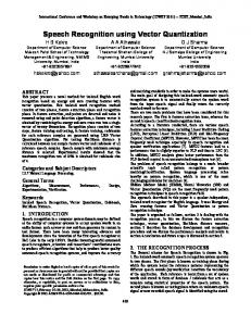
Fig. 1. Block diagram of the proposed EMG-based ASR system. Top: Offline (training) procedure. Bottom: Online (recognition) procedure.

susceptible to temporal variations [9]. In [8], a linear discriminant analysis (LDA) accompanied by a principle component analysis (PCA) was carried on the time-normalized AR coefficients to recognize the number of single (isolated) digits. The authors indicated that LDA-based recognition was less robust than the HMM-based approach [7]. Since voices are created using various articulatory muscles, multichannel EMG signals would be highly desirable in order to increase classification performance. Accordingly, the state observation density of HMM is represented with multiple observations from multichannel EMG signals. In this paper, we focus on modeling and integrating the multichannel EMG signals. We first define a model that describes the relationship between the features from the multichannel EMG signals and a model training method is then developed. Our assumption is that the occurrence of observations for each EMG channel is controlled by both intra/inter probabilistic models. The term intra means that an underlying probabilistic model affects intrachannel variabilities. Whereas interchannel variabilities are affected by an inter probabilistic model. In the proposed method, intra/inter probabilistic models are represented by a Gaussian mixture model (GMM), and cross correlational probabilities, respectively. The cross correlational probability density functions for each channel commonly include the one shared random variable, which is referred to as the global control variable (GCV). This means that the occurrences of observations for each EMG channel are globally controlled by the GCV. The parameters for representing each probabilistic model are obtained by means of a maximum likelihood (ML) estimation. The state observation densities of the underlying HMM are derived from the proposed probabilistic model. The proposed method is somewhat different from the method based on an independent model [2], where interchannel dependencies are not taken into consideration in representing the state observation densities. It is known that EMG signals detected via the skin are mixtures of contributions generated by all the active muscles when two or more muscles close to each other are simultaneously active [3]. Moreover, it can be said that the facial muscles are inherently controlled by a command from the brain. These can be thought of as the evidence of statistical dependencies between multichannel EMG signals.

Hence, it would be expected that the inter/intra channel model is ideally-fitted for HMM under conditions where multichannel EMG signals are given, and would eventually increase recognition accuracy. To evaluate the validity of the proposed model, we performed several experiments designed for the recognition of 60 isolated words. The results were compared with the different models (including the independent model and the feature-domain dependent model) II. OVERVIEW OF THE EMG-BASED ASR SYSTEM A block diagram of the proposed EMG-based ASR system is shown in Fig. 1. There are two stages; In the training stage (off-line stage), EMG signals are first obtained, an analysis is performed on these EMG samples to derive the feature parameters to be used as input signals for the ASR system. The parameters describing HMM are estimated using the features from the EMG signals and their orthgraphic word transcription. In the online stage, the feature parameters which are identical to those in the training stage are derived from the incoming EMG signals. The feature parameters are then fed into the recognition procedure, which is based on a maximum likelihood (ML) estimation. Each part of the proposed system is described in more detail in the following sections. A. EMG Detection Since there is no explicit relationship between the functions of each facial muscle and recognition performance, it is very difficult to find the optimal locations of the facial muscles in the sense of maximizing recognition accuracy in an analytical way. Hence, the locations of EMG electrodes were determined heuristically, based on a trial-and error approach. In this work, surface EMG signals were obtained from three articulatory muscles of the face: the levator anguli oris, the zygomaticus major, and the depressor anguli oris. The levator anguli oris originates from canine fossa immediately below the infraorbital of the maxilla (bone) and has a role in raising the skin tissue upwards from the corners of the mouth. The zygomaticus major originates from the zygomatic bone, and has a role in drawing the angle of the mouth upward and outward. The depressor anguli oris originates from the mandible and inserts skin at an

932


angle of mouth and pulls corner of mouth downward. A detailed description of EMG detection is found in Section IV

obtained by summing the joint probability (2) over all possible state sequences , giving

B. Feature Parameters

(3)

The features are extracted from the windowed EMG signals. A 100 msec length Hanning window was used to compute and extract the feature parameters at 20 msec intervals. The log melfilter bank channel output was adopted, which is given by the output of the mel scale filter bank. The mel scale is given by (1) where is frequency in hertz. Mel-scale filter bank analysis reflects the human auditory system [13]. Although an EMG signal is not perceived by the human ear, the usefulness of mel-scale filter bank analysis has been confirmed in several EMG-based ASR systems [2], [10]. For most ASR systems, other useful features include the first and second temporal derivatives of the feature vector called the delta and delta-delta (acceleration) coefficients, respectively. These derivatives help give an estimate of the temporal variations in the signal and can be applied to the underlying EMG-based ASR system. However, the experimental results showed that performance improvement was not remarkable when acceleration coefficients were adopted. Accordingly, in our approach, only delta coefficients were employed in HMM estimation and recognition. C. Hidden Markov Model-Based Word Recognition The HMMs represent a stochastic process that takes time series data as the input, and outputs the probability that the data is generated by the model. HMMs have been successfully employed in many speech recognition tasks [14], [20]. An HMM is comprised of states, with each state containing a state ob, which determines the servation probability distribution likelihood of generating observation in state at time . The probability of an observation moving from state to state is defined by the transition probability . The state observation probability is represented as a multivariate Gaussian distribution (continuous density HMM) or discrete distribution (discrete density HMM). , Given independent observations , and the model dea state sequence scribing HMM, the probability that and occur simultaneously is given by

Now, the problem of HMM parameter estimation can then be formulated as follows: (4) i.e., finding the HMM parameters in which the likelihood of the underlying model can be maximized, given the training data. This maximization problem can be solved by the Baum–Welch reestimation formulas, based on the expectation-maximization (EM) algorithm [17]. A different optimization criterion for estimating the parameters of the HMM was devised by Juang et al. [21]. In this method, the HMM parameters are estimated by maximizing the state-optimized likelihood. Hence, the optimal HMM parameters are given by (5) This method is known as the segmental -means algorithm [21]. In this algorithm, the HMM parameters for the th state of the th word are estimated from observations belonging to the corresponding state of the same word. Accordingly, prior to estimating the HMM parameters, segmentation should be performed to obtain state boundaries. The sequence of the states can be automatically obtained by a forced-alignment technique [21]. Since the segmental -means algorithm does not take into account a state sequence having a very low likelihood, numerical difficulties can be avoided which are frequently encountered when the Baum–Welch reestimation algorithm is used. After constructing a set of HMMs for all words to be recognized, recognition is performed by finding a word template that yields the maximum likelihood of the incoming observation sequence (6) the maximum likewhere denotes the word’s HMM and lihood word template (or recognized word template) Since the is evaluated for all possible words, maxilikelihood mization (6) requires a huge amount of computation. To reduce the number of computations, Viterbi decoding [14] is frequently employed to solve the problem (6). III. HIDDEN MARKOV MODEL FOR MULTICHANNEL OBSERVATION

(2) . If the number of states is , there are where such state sequences. The probability of (given the model) is

A. Model It is known that a number of articulatory facial muscles are involved in producing speech [5]. Hence, it would be desirable that an observation vector could be composed of a number


933

of individual feature vectors obtained from different facial muscles. There are several methods available for integrating the individual feature vectors. They can be divided into early integration (EI) and late integration (LI) models [12]. In the EI model, integration is performed in the feature space to form a composite feature vector for the multiple features for each channel. Hence, a state observation density is given by the probability of this composite feature vector. In the LI model, a density function is defined for each feature. A state observation density is then represented by integrating individual density functions. The focus of this paper is on the LI model. One simple way of implementing the LI model is to assume that all the individual density functions are statistically independent. In this case, a state observation density is given by (7) denotes the density function for the th channel where denotes the total number of EMG chanfeature vector and nels. In (7), the state index is omitted for simplicity. When the Gaussian mixture model is adopted, an individual density function is given by (8) where is the number of Gaussians for the th channel observation and is the mixture weight for the th Gaussian is the th Gaussian component for the component. th channel, that is

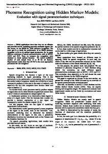
Fig. 2. Graphical depiction of the proposed model for representing the state , , and observation density. (In the case of the state index ).

where

(9) where and are the covariance matrix and mean vector of the th Gaussian random source for the th channel feature is the order of the th channel feature vector, respectively. vector . Using (8) and (9), a state observation density is given by (10) is the number of Gaussian components for the th where is channel observation vector. the joint probability function of the set of the observation vecand the set of the Gaussian random sources tors , which is given by (11) This model does not take into account interchannel dependencies that may exist in multichannel EMG signals. We define the following state observation density function that reflects interchannel dependencies (12)

Compared with the independent model (11), the mixture are replaced with conditional probabilities weights . This implies that the occurrences of each observation vector are partly controlled by the random source , as shown in Fig. 2. Since this random source is commonly involved with all of the mixture weights, we refer to this random source as a global control variable (GCV). In other words, the dependencies between the multichannel observations are described by adopting the correlational probabilities with the is the common (or sharing) random variables. Note that number of the GCVs in (12). The state observation density involved with GCV is given by

(13) Note that the state observation densities (10) and (13) are . This imidentical in the case of plies that the state observation density without interchannel dependencies is a special case of the proposed model, where the and GCV are statistically inGaussian random source and . Hence, it can dependent for be said that the proposed model yields a more generalized form of the state observation density function, compared to the independent model.

934


B. Maximum Likelihood Parameter Estimation In this paper, HMM parameters are estimated in the framework of the segmental -means algorithm. This method segments each training token into states by determining the optimal (Viterbi) alignment of the current model with each training token. All observations for a given word, in a given state, are used as inputs to a model training algorithm for the corresponding state of the word. Since the optimal model parameters (or optimal state sequences) should be reestimated with the given state sequences (or model parameters ), state segmentation and model training are performed iteratively. , The goal of model training is to estimate and parameters describing , for and which, in some sense, best matches the acof the training tual distribution feature vectors. To this end, the ML estimation is employed in this work. The aim of ML estimation is to find the model parameters in which the likelihood of the underlying probabilistic model can be maximized, given the training data. For a sequence of multichannel training vectors , the likelihood function of parameter set over can be written as

where

trix are estimated independently using the clusters obtained by , VQ for each training vector set . The other parameters (the cross correlational probabilities , , , and the probabilities , ) are randomly initialized, under of GCV the constraint wherein the sum of the probabilities is unity. For the remaining HMM parameters (state transition probaand initial probability ), the method proposed by bility Rabiner et al. [20] was adopted in this study. C. Pruning In order to improve the generalization of the model, it would be useful to penalize a cross correlational probability that has a low frequency. A possible way of accomplishing this is to replace the probability estimate used above by the lower bound of is replaced the confidence interval of this estimate, i.e., by (17) where

(14)

(18)

with , is a particular sequence of random sources. is given by

(19)

(15) Hence, the notation denotes the sum over all possible random source sequences. The optimal parameter set is given by (16) Since the likelihood function (14) is a nonlinear function of the parameters , a direct maximization cannot be achieved. However, ML parameter estimates can be obtained iteratively using a special case of the expectation-maximization (EM) algorithm [17]. The basic concept of the EM algorithm is, beginning with an initial model , to estimate a new model , such that . The new model then becomes the initial model for the next iteration and the process is repeated until an acceptable convergence threshold is reached. The reestimation formulas used in each EM iteration are presented in appendix . An important implementation issue associated with the EM algorithm is its initialization. In practice, the initialization of the EM algorithm affects its convergence rate but can also modify the final result [17]. In this study, the model parameters are initialized by the use of a standard full-search vector quantization (VQ) procedure [18]: a mean vector and a covariance ma-

is omitted for the sake of simplicity. The channel index , is the lower bound of With pruning factor , the 95% confidence interval. When is set to 0. With such an estimate, the sum of the probabilities reaches a value lower than 1, which requires renormalization. IV. METHOLOGY Eight male Korean subjects participated in this study. A 60-word vocabulary consisting of the words listed in Table I was used. The list is phonetically balanced, which means it has speech sounds, or phonemes, that occur as often as they would in a normal conversation. The subjects were asked to pronounce each word in a consistent manner, minimizing variations in volume and speaking style. A set of words is composed of the sixty words in Table I. The order of the words in each set was randomly permuted. For each subject, the training corpus and the test corpus include 1500 words (25 sets) and 900 words (15 sets), respectively. The location of each electrode for each muscle is shown in Fig. 3. Each EMG signal was collected using pairs of Ag–AgCl button electrodes (3M, 2258). The electrodes were 3.3 cm in diameter (including the foam adhesive patch). The active area of the electrode is about 1.5 cm in diameter. For each electrode pair, the distance between the centers of each electrode was of 2 cm. The reference electrode was located at the back of the neck. Before acquiring the EMG signals, the EMG target locations were cleaned with alcohol wet swabs. A preamplifier (with a Gain of 1000) was placed for each EMG channel, which was implemented by a high-precision instrumentation amplifier (Analog Device, AD620). To minimize


935

TABLE I LIST OF THE WORDS

Fig. 3. Locations of electrodes for detecting EMG signals of articulatory facial muscles: A: levator anguli oris; B. depressor anguli oris; C. zygomaticus major.

motion artifacts and aliasing, a bandpass filter (with low corner ( 3 dB) 10 Hz and with high corner ( 3 dB) frequency of 300 Hz) was used. To increase robustness against power line noise, a notch filter (with a notch frequency of 60 Hz) would be desirable. However, since it is known that the dominant energy of EMG lies in the 50–150 Hz range [4], a coarsely designed analog notch filter would affect the performance of the under-

lying ASR system. Hence, the notch filter was implemented in the digital domain, with the advantage of high cut-off characteristics. The EMG signal was sampled at 8000 Hz with 16 bit precision (Cyruss Logic, CS5330A), then down sampled at 1000 Hz. Digital data were transmitted over a universal serial bus (USB) to a desktop PC with a Pentium D-processor. The number of mel-scale filter channels for the parameters is 5, determined under the constraint that the highest center frequency of the filter bank is less than the Nyquist frequency ). The feature vector is composed of the features from ( the three EMG channels and their delta features. Hence, the total number of EMG feature parameters for defining HMM is 30. In training the HMM parameters, a typical left-to-right model was used. The distribution of acoustic features were modelled using mixtures of diagonal Gaussians. The number of states for each word’s HMM was determined heuristically, and was five. V. RESULTS A. The Average Likelihood for Each Model Prior to evaluating the performance in terms of recognition, we first evaluated how well each model matches the real EMG of the given data. To this end, the average likelihoods training/test data with respect to the underlying model were computed. The EI model, the independent LI model and the dependent LI model (proposed) were all evaluated. For the inde-

936


Fig. 4. Average log likelihoods for each model, according to the number of Gaussians.

TABLE II Two-WAY ANOVA TABLE FOR THE AVERAGE LOG LIKELIHOODS. TOP: BETWEEN THE EI MODEL AND THE LI-GCV MODEL, BOTTOM: BETWEEN THE LI-INDEPENDENT MODEL AND THE LI-GCV MODEL

pendent LI model, the model training method employed in [19] was adopted, which is based on a maximum likelihood criterion. For the EI model, the state observation densities of the all the states over all the words were estimated from the integrated feature vectors. The number of the GCVs in the dependent LI model was set to the value that yields the highest recognition rate. Since the parameters for all models are obtained by an iterative algorithm, the final likelihood may be affected by the initialization method employed and the number of iterations used. Since the proposed training method for the dependent LI model is based on VQ-based initialization, the same approach was also employed in initializing the parameters for the EI model and the independent LI model. We also employed ) in the iteration algoa sufficiently small threshold ( rithm that tends to produce more stable results. The results are shown in Fig. 4. For the LI models, the average log likelihoods increased monotonically as the number of Gaussians increased. All three models yield similar trends with increasing number of Gaussians. This is due to the fact that a maximum likelihood criterion was commonly employed in all model training methods. However, the average log likelihoods of the dependent LI model were consistently higher than the other models. As shown in Fig. 4, the differences in the average log likelihood between the EI model and the dependent LI model are more remarkable than those between the independent LI model and the dependent

LI model. This is also confirmed by the two-way ANOVA test, which is shown in Table II. The -value of the model factor is ) when the the EI-model and dependent LI model 0.01 ( ) was obare considered. Whereas, the -value of 0.432 ( served in the ANOVA test when the underlying models include the LI-independent and the LI-dependent mode. Comparing the -values of the number of Gaussians (0.014 and 0.01, ) and those of the model, it can be understood that the major factor to affect the average log likelihood is the model employed, when the underlying models include the EI model and the dependent LI model. B. Recognition Accuracy According to the Number of Gaussians Fig. 5 plots the average word recognition rate (WRR) for the EI model and the dependent LI model, along with the dependent LI model, for comparison. The number of the GCVs in the dependent LI model was also set to the value that yields the highest recognition rate. The dependent LI model consistently produced higher WRR than the independent LI model, which would be expected as the average log likelihood of the dependent LI model is always higher than the independent LI models. Even when the number of Gaussians for the dependent LI model is smaller than that of the independent LI model, the WRR of the dependent LI model is lower than that of the independent LI model. The difference in WRR between the dependent LI model and the independent LI model increases as the number of Gaussians is increased, until the number of Gaussians reaches four. The two models show different trends with increasing number of Gaussians. For the dependent LI model, WRR is monotonically increased until the number of Gaussians reaches four. For the independent LI model, however, WRR does not significantly change until the number of Gaussians reaches four. According to our experiments, there is no explicit relationship between the number of Gaussians and WRR. This is also confirmed by the two-way ANOVA test, shown in Table III. In this table, the number of Gaussians does not significantly affect the average , ). Whereas the underlying model is WRR ( , ). the key factor to affect the average WRR ( Although the LI models (both the independent and dependent models) always yielded a higher average likelihood than the EI model, the average WRR for the EI model are higher than the independent LI models. The average WRR for the dependent LI model is slightly higher than that of the EI model. As shown in Fig. 5, the WRR for the EI model and the dependent LI model increases monotonically until the number of Gaussian reaches four. Hence, the best recognition was achieved when the number of Gaussians was set at four in Fig. 5. The difference in the highest average WRR between the EI model and the dependent LI model is 0.36% (87.0% versus 86.64%). This difference is not so remarkable, compared with the difference between the independent LI model and the dependent LI model. The two-way ANOVA test (Table III) also shows that the average WRR is not , so significantly affected by the model employed ( ), when the underlying model includes the EI model and the dependent LI model.


937

TABLE IV INTER-SUBJECT VARIABILITIES IN WORD RECOGNITION RATE (WRR)

Fig. 5. Recognition rate as a function of the number of Gaussians.

TABLE III Two-WAY ANOVA TABLE FOR WORD RECOGNITION RATES. TOP: BETWEEN THE EI MODEL AND THE LI-GCV MODEL, BOTTOM: BETWEEN THE LI-INDEPENDENT MODEL AND THE LI-GCV MODEL

Fig. 6. Recognition rate as a function of the number of GCVs.

The intersubject variabilities were also observed in this work. The results are summarized in Table IV. For the independent LI model, the standard deviation between the subjects is relatively higher than other models. The EI model has the lowest standard deviation. This means that the EI model yields the more consistent performance in terms of recognition accuracy. It was also observed that the trends of the highest WRR and the lowest WRR among the subjects are similar to those of the average WRR.

TABLE V Two-WAY ANOVA TABLE FOR WORD RECOGNITION RATES, FACTOR: THE NUMBER OF GCVS AND THE NUMBER OF GAUSSIANS

C. Recognition Accuracy According to the Number of GCVs The accuracy of recognition may be affected by the number of the GCVs in the dependent LI model, as well as by the number of Gaussians. Hence, the issue of how recognition accuracies are affected by the number of the GCVs in the dependent LI model, under the conditions where the number of Gaussians is fixed is of interest. Fig. 6 shows the average WRRs for different numbers of GCVs. The WRR of the dependent LI model shows no definite trend with increasing number of GCVs. The two-way ANOVA test also shows that there is no relationship between the average WRR and the number of GCVs, which is shown in Table V. The -value of the factor “the number of GCVs” ), which means that the average WRR is not is 1.000 ( affected by the number of GCVs. Comparing with the -value of the factor “the number of Gaussians” ( , ), the

number of the Gaussians can be regarded as a key factor to affect the recognition accuracy. This result is somewhat different from the previous ANOVA test results (Table III), where the signifi, cance of the number of Gaussians is relatively lower ( , ). A possible explanation for this inconsistent result is that the average WRRs for all possible number of GCVs were taken into consideration in Table V. However, only one GCV number was considered in the ANOVA test results from Table III. D. Recognition Accuracy With/Without Pruning Thus far, all results of the dependent LI model were obtained in cases when pruning was employed in model training. In this

938


WRRs are almost identical, when the number of GCVs is small. The ANOVA test was conducted for the results in the case of all possible GCV numbers (2 9). So, it can be expected that the significance of the factor “pruning” is increased when relatively large number of GCVs is exclusively adopted. VI. DISCUSSION

Fig. 7. Recognition rate with/without pruning (In case of No. of Gaussians ).

TABLE VI Two-WAY ANOVA TABLE FOR WORD RECOGNITION RATES. FACTOR: PRUNING/NO PRUNING AND THE NUMBER OF GCVS

section, we investigate the contribution of pruning in model training to recognition accuracy by comparing the results from the two HMMs obtained by model training methods with/without pruning, respectively. Fig. 7 shows plots of the average WRRs for different numbers of GCVs, along with the average WRR from the HMM obtained using model training without pruning. The results were obtained when the number of Gaussians was 4. The overall trend with different numbers of GCVs is consistent with previously obtained results (in the case of with pruning). However, it appears that recognition performance is improved by employing model training with pruning. However, the difference in the average WRR is not so ). significant, when the number of GCVs is relatively small ( Fig. 7 also shows that, as the number of GCVs is increased, the differences in average WRR between with and without pruning are increased. Accordingly, the average WRR is significantly reduced when the model training method with pruning is used, ) is employed. This suggests when the maximum GCVs ( that the use of pruning in model training is desirable, especially when the number of GCVs is large. A statistical significance test was also conducted to demonstrate how much the experimental test results are statistically meaningful. Table VI is the two-way ANOVA table for the average recognition rate, which includes the two factors: the number of GCVs and with/without pruning. The value of ) was obtained from Table VI. This value does 0.637 ( not clearly reject the null hypothesis (pruning and nonpruning training methods are independent in terms of the average WRR). A possible explanation for this result is that the average

There are several ways to prove the evidence of the dependencies among the multichannel streams. Mutual entropy [22] is one of them. Since multichannel EMG data is regarded as time-varying random sources, the dependencies among the multichannel streams are measured in the HMM framework. Our results show that dependencies exist among the multichannel EMG signals, which was confirmed by the results from likelihood tests and recognition tests. For the likelihood test, the dependent LI model was shown to be the best matched with the actual multichannel EMG data. There are two possible reasons for this higher average likelihood of the dependent LI model, compared with the independent LI models and the EI model. First, a larger number of parameters describing the dependent LI model than the independent LI model were used, because a number of GCVs are added to the parameters of the dependent LI model. Since the GCVs are estimated by maximizing the overall likelihood of the training corpus, these additional features also contribute to an increase in overall likelihood. Indeed, it was observed that as the number of GCVs was increased, the average likelihood of the independent LI model was also increased when the number of Gaussians was fixed. The other reason for the higher likelihood of the dependent LI model can be explained by the dependencies among the multichannel EMG signals. It is noteworthy that, since the feature parameters of the EI model are given by integrating all the individual channel parameters, it can be said that the channel dependencies are implicitly taken into consideration in the EI model. Nevertheless, the average likelihoods for the EI model are always lower than those for the other models. This can be also explained by the fact that the number of parameters for describing the EI model is smaller than the other models. For example, when the number of EMG channels and the number of Gaussians are 3 and 4, respectively, the number of the mixture weights for the EI model is 4 and 12 for the LI-model. (The number of variables representing the mean vectors and the covariance matrices are the same.) Assuming that the overall likelihood is reduced by increasing the number of parameters for describing the underlying model, a low likelihood for the EI-model is not an unexpected result. Although the model parameters are optimal from the standpoint of the maximum likelihood criterion, it does not necessary mean that the higher likelihood parameter always yielded the better performance in terms of recognition accuracy. This was confirmed by the results shown in Fig. 5, where the EI model, which resulted in the least likelihood, yielded the higher WRR than the independent LI model. However, the performance of the dependent LI model in recognition accuracy is always higher than than of the EI model, except when the number of Gaussians is two. (two models have identical recognition rates) The differences in recognition accuracy between the EI model and the dependent LI model were not remarkable, which was confirmed by


the two-way ANOVA test. This means that the maximum likelihood criterion employed in GCV estimation could be replaced by other criteria. The minimum classification error (MCE) criterion [23] or the maximum mutual information (MMI) criterion [24] can be taken into consideration for further increasing the recognition accuracy. Recognition accuracy was affected by pruning employed in model training. Maximally, the average WRR was increase by 1.0% when the HMM parameters derived from the training method involved pruning. We confirmed that the application of pruning often led to a remarkable improvement in recognition accuracy, especially when the number of GCVs is large. A possible explanation for this improved performance is that, smaller (or noisy) correlational probabilities are merged with larger correlation probabilities by applying pruning in model training. This resulted in an increased generality of the model. As the number of GCVs is increased, the number of possible combinations of GCVs and Gaussian variables also increased. This tends to produce many small conditional probabilities, which reduces the generality of the model. Hence, the benefits of using pruning in model training are more remarkable when a larger number of GCVs is employed. This was confirmed by the results shown in Fig. 7.

939

APPENDIX MODEL TRAINING For each EM iteration, the following reestimation formulas are used which guarantee a monotonic increase in the model’s likelihood value. Cross Correlational Probability:

(20)

where

Probability of Global Control Variable:

(21) where

VII. CONCLUSION In this work, an EMG-based ASR scheme is proposed and the performance of the proposed scheme was evaluated. Our interests are mainly focused on the representation of the state observation probabilities. The underlying assumption is that interchannel dependencies exist among the features derived from the multichannel EMG data. The dependencies were represented using cross correlational probabilities between individual channel data and global control variables. Several related issues including model parameter estimation were also proposed, based on a maximum likelihood criterion. The findings here show that HMM derived from the dependent model produced better recognition accuracy than the independent model. This was confirmed by experimental results, yielding up to an 85.07% recognition accuracy where recognition was performed on the isolated words. The resultant recognition accuracy of the proposed model is comparable with that of the early integration model. The proposed approach can be applied to the other multichannel ASR schemes, such as audio-visual ASR systems. To increase the usefulness of the EMG-based ASR system, some practical aspects should be considered. For example, the number of words to be recognized should be increased. Moreover, the system can recognize more complicated sentences which are often used in real-life situations. Another weak point of the proposed scheme is that the locations of electrodes were not determined optimally. Hence, a detailed analysis of the relationship between the function of each facial muscle and the phonemes spoken would be desirable. This will provide clues for determining the optimal locations for collecting the surface EMG signals. Our future studies will focus on these issues.

Mean Vectors:

(22)

where

Covariance Matrices:

(23)

where

The a posteriori probabilities are given by

(24)

940


(25)

(26) REFERENCES [1] S. Kumar, D. K. Kumar, M. Alemu, and M. Burry, “EMG based voice recognition,” in Proc. IEEE ISSNIP, 2004, pp. 597–596. [2] H. Manabe and Z. Zhang, “Multi-stream HMM for EMG-based speech recognition,” in Proc. 26th Ann. Int. Con. IEEE EMBS, San Francisco, CA, 2004, pp. 4389–4392. [3] D. Farina, C. Fevotte, C. Doncarli, and R. Merletti, “Blind separation of linear instantanous mixtures of nonstationary surface myoelectic signals,” IEEE Trans. Biomed. Eng., vol. 51, no. 9, pp. 1555–1567, Sep. 2004. [4] K. Ogino and W. M. Kozak, “Spectrum analysis of surface electromygram,” in Proc. IEEE Int. Conf. Acoustic, Speech, Signal Processing, Boston, MA, 1983, pp. 1114–1117. [5] F. Grandori, P. Pinelli, P. Ravazzani, F. Ceriani, G. Miscio, F. Pisano, R. Colombo, S. Insalaco, and G. Tognola, “Multiparametric analysis of speech production mechanisms,” IEEE Eng. Med. Biol., vol. 4–5, no. 2, pp. 203–209, Apr./May 1994. [6] H.-J. Park, S.-H. Kwon, H.-C. Kim, and K.-S. Park, “Adaptive EMGdriven communication for the disability,” in Proc. 1st Joint BMES/ EMBS Conf. Serving Humanity, Advancing Technology, Atlanta, GA, 1999, p. 656. [7] A. D. C. Chan, K. B. Englehart, B. Hudgins, and D. F. Lovely, “Hidden Markov model classification of myoelectics signals in speech,” IEEE Eng. Med. Biol., vol. 9–10, no. 5, pp. 143–146, Sep./Oct. 2002. [8] A. D. C. Chan, K. B. Englehart, B. Hudgins, and D. F. Lovely, “Myoelectric signals to augment speech recogntion,” Med. Biol. Eng. Comput., vol. 39, no. 4, pp. 500–504, 2001. [9] A. D. C. Chan, K. B. Englehart, B. Hudgins, and D. F. Lovely, “Multiexpert automatic speech recognition using acoustic and myoelectric signals,” IEEE Trans. Biomed. Eng., vol. 53, no. 4, pp. 676–685, Apr. 2006. [10] K.-S. Lee, “HMM-based automatic speech recognition using EMG signals,” J. Biomed. Eng. Res. (J-BME), vol. 27, no. 3, pp. 101–109, Jun. 2006. [11] R. S. Kumaran, K. Narayanan, and J. N. Gowdy, “Myoelectric signals for multimodal speech recognition,” in Proc. INTERPEECH (Eurospeech), Lisboa, Portugal, 2005, pp. 1189–1192. [12] A. Q. Summerfield, “Lipreading and audio-visual speech perception,” Philos. Trans. R. Soc. London B, vol. 335, pp. 71–78, 1992.

[13] L. R. Rabiner and R. W. Schafer, Digital Processing of Speech Signals. Englewood Cliffs, NJ: Prentice-Hall, 1978. [14] L. R. Rabiner and B. H. Juang, Fundamentals of Speech Recognition. Englewood Cliffs, NJ: Prentice-Hall, 1993. [15] G. M. White and R. B. Neely, “Speech recognition experiments with linear prediction, bandpass filtering, and dynamic programming,” IEEE Trans. Acoust. Speech Signal Process., vol. ASSP-24, no. 2, pp. 183–188, Apr. 1976. [16] C. Jorgensen, D. D. Lee, and S. Agabon, “Sub auditory speech recognition based on EMG signals,” in Proc. Int. Joint Conf. Neural Netw., 2003, vol. 4, pp. 3128–3133. [17] A. Dempster, N. Laird, and D. Rubin, “Maximum likelihood from incomplete data via the EM algorithm,” J. Royal Stat. Soc., vol. 39, pp. 1–38, 1977. [18] Y. Linde, A. Buzo, and R. M. Gray, “An algorithm for vector quantizer design,” IEEE Trans. Communications, vol. 28, no. 1, pp. 84–95, Jan. 1980. [19] D. A. Reynolds and R. C. Rose, “Robust text-independent speaker identification using Gaussian mixture speaker models,” IEEE Trans Acoust. Speech Signal Process., vol. 3, no. 1, pp. 72–83, Jan. 1995. [20] L. R. Rabiner, J. G. Wilpon, and F. K. Soong, “High performance connected digit recognition using hidden Markov models,” IEEE Trans. Acoust., Speech Signal Process., vol. 37, no. 8, pp. 1214–1225, Apr. 1989. [21] B.-H. Juang and L. R. Rabiner, “The segmental -means algorithm for estimating paramters of hidden Markov model,” IEEE Trans. Acoust., Speech Signal Process., vol. 38, no. 9, pp. 1639–1641, Sep. 1990. [22] Q. Hongzhi, W. Baikun, and L. Zhao, “Mutual information entropy research on dementia EEG signals,” in Proc. 4th Int. Conf. Computer and Information Technology, 2004. CIT ’04, Sep. 2004, vol. 14–16, pp. 885–889. [23] G. Potamianos, C. Neti, G. Gravier, A. Garg, and A. W. Senior, “Recent advances in the automatic recognition of audiovisual speech,” Proc. IEEE, vol. 91, no. 9, pp. 1306–1326, Sep. 2003. [24] L. R. Bahl, P. F. Brown, P. V. deSouza, and L. R. Mercer, “Maximum mutual information estimation of hidden Markov model parameters for speech recognition,” in Proc. IEEE Int. Conf. Acoustic, Speech, and Signal Processing, Tokyo, Japan, Apr. 1986, pp. 49–52. Ki-Seung Lee was born in Seoul, Korea, in 1968. He received the B.S., M.S., and Ph.D. degrees in electronics engineering from Yonsei University, Seoul, Korea, in 1991, 1993, and 1997, respectively. Since September 2001, he has been an Assistant Professor at Konkuk University, Seoul, Korea. From February 1997 to September 1997, he was with the Center for Signal Processing Research (CSPR) at Yonsei University. From October 1997 to September 2000, he was with the Speech Processing Software and Technology Research Department, Shannon Laboratories, AT&T Laboratories-Research, Florham Park, NJ, where he worked on ASR/TTS-based very low bit rate speech coding and prosody generation of the AT&T TTS Systems. From November 2000 to August 2001, he was with the Human and Computer Interaction Laboratories, Samsung Advanced Institute of Technology (SAIT), Suwon, Korea, where he worked on a corpus-based TTS System. His interests include bio-signal recognition, electromyogram-to-voice conversion, prosody control of automatic speech synthesis system, voice conversion and image enhancement.