automatic speech recognition using hidden conditional ... - CiteSeerX

AUTOMATIC SPEECH RECOGNITION USING HIDDEN CONDITIONAL NEURAL FIELDS Yasuhisa Fujii, Kazumasa Yamamoto, Seiichi Nakagawa Toyohashi University of Technology Department of Computer Science and Engineering 1-1 Hibarigaoka, Tenpaku-cho, Toyohashi, Aichi 441-8580, JAPAN ABSTRACT Hidden Conditional Random Fields(HCRF) is a very promising approach to model speech. However, because HCRF computes the score of a hypothesis by summing up linearly weighted features, it cannot consider non-linearity among features that will be crucial for speech recognition. In this paper, we extend HCRF by incorporating gate function used in neural networks and propose a new model called Hidden Conditional Neural Fields(HCNF). Differently with conventional approaches, HCNF can be trained without any initial model and incorporate any kinds of features. Experimental results of continuous phoneme recognition on TIMIT core test set and Japanese read speach recognition task using monophone showed that HCNF was superior to HCRF and HMM trained in MPE manner. Index Terms— hidden conditional neural fields, hidden conditional random fields, HMM, speech recognition 1. INTRODUCTION Current ASR systems employ Hidden Markov Model(HMM) with Gaussian Mixture Model(GMM) as emission probability for acoustic model. However, HMM has two major drawbacks to use for acoustic model. Firstly, HMM has a strong independency assumption that frames are independent given a state, thus, lacks an ability to deal with a feature which straddles over several frames. Secondly, because HMM is a generative model, it is not suitable to discriminate sequences. To solve the former problem, features that can deal with phenomena straddling over frames have been developed such as delta coefficient [1], segmental statistics [2] and modulation spectrum [3]. For the latter problem, discriminative training methods like MPE have been investigated [4]. Combining a model that can consider long range features and has high discriminative power with HMM has also been conducted to tackle above problems. For example, Tandem system extracts features using Multi Layered Perceptron(MLP) and utilizes them as an input for HMM [5]. Conditional Random Fields(CRF) [6] also could be used instead of MLP [7]. Hidden Conditional Random Fields (HCRF) is a very promising approach to model speech [8, 9, 10]. HCRF overcomes two major drawbacks of HMM mentioned above while This work was supported by Global COE Program Frontiers of Intelligent Sensing from the Ministry of Education,Culture,Sports, Science and Technology, Japan.

978-1-4577-0539-7/11/$26.00 ©2011 IEEE

5036

preserving the merits of HMM such as efficient algorithms including forward-backward algorithm and Viterbi decoding. Although HCRF is promissing, it still has a drawback that it cannot consider non-linearity among features which would be crucial for speech recognition because it computes the score of a hypothesis by summing up linearly weighted feature values. There is an attempt to expand feature vectors explicitly [11]. However, it will be difficult to use the approach when the number of features increases. Peng et al. proposed Conditional Neural Fields(CNF) which can consider non-linearlity among features by incorpolating gate function into CRF[12]. In this paper, we propose Hidden Conditional Neural Fields(HCNF) which can consider non-linearlity beween features by introducing gate function into HCRF. Differently with conventional approaches, HCNF can be trained without any initial model and incorporate any kinds of features. Although it seems that our work is close to the work presented in [13], their work extended CRF to incorpolate gate function, and thus, it was close to CNF rather than our work. Experimental results on continuous phoneme recognition on TIMIT core test set and Japanese read speech recognition task show that HCNF is superior to HCRF and HMM trained in MPE manner. This paper is organized as follows. In the next section, HCRF for ASR is described. After that, HCNF is introduced in Section 3. In Section 4, the training methods for HCRF and HCNF are explained. The experimental setup and results are shown in Sections 5. Finally, Section 6 presents our conclusions and some future works. 2. HIDDEN CONDITIONAL RANDOM FIELDS 2.1. Formulation Given a observation sequence X = (x1 , x2 , . . . , xT ), HCRF computes a score of a label sequence Y = (y1 , y2 , . . . , yT ) as follows: P (Y |X) =

1  exp(κ(Φr (X, Y, S) + Ψr (X, Y, S))), Z(X) S (1)

where κ is a state-flattening coefficient [14]. Z(X) is a partition function and computed as follows: Z(X) =

 Y

exp(κ(Φr (X, Y, S) + Ψr (X, Y, S))),

(2)

S

ICASSP 2011

Φr (X, Y, S) and Ψr (X, Y, S) are an obseration function and a transition function, respectively, and defined as follows: Φr (X, Y, S) =





φk (X, Y, S, t),

(3)

ψj (X, Y, S, t, t − 1).

(4)

t

k

Ψr (X, Y, S) =



wk uj

 t

j

S = (s1 , s2 , . . . , sT ) is a hidden variable sequence that represents a state sequence. φk (X, Y, S, t) and ψj (X, Y, S, t, t − 1) mean a raw observation feature extracted at frame t and a transition feature extracted at frame t and t − 1, respectively. Corresponding weights are wk and uj , respectively. Because the feature functions used in HCRF are restricted to current frame in the observation function, and current and previous frames in the transition function, efficient algorithms such as forward-backward algorithm and Viterbi algorithm can be adapted to HCRF.

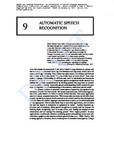
(a) HCRF

(b) HCNF

Fig. 1. The structure of HCRF and HCNF. where φ(X, Y, S, t) is a vector representation of φk (X, Y, S, t) in Eq.(3) and θy,s,g is a corresponding weight vector specific to the triple of y, s and g 1 , h(x) is a gate function defined as follows:

2.2. Training

1 − 0.5. 1 + exp(−x)

h(x) = i

i

Given training data D = {X , Y }, i = 0, . . . , N , the objective function of HCRF is set as follows: l(λ; D) = −



log P (Y i |X i ).

(5)

i

In HCNF, the observation function Φn (X, Y, S) uses K gate functions by which it considers non-linearlity among features. Using Eqs.(7) and (8), P (Y |X) can be computed as follows:

λ = {wk , uj } which minimizes l(λ; D) can be found using gradient based methods such as L-BFGS and Stochastic Gradient Descent(SGD). The partial derivatives of Eq.(5) with respect to wk can be computed as follows:     ∂l(λ; D) =−κ E φk (X i , Y i , S, t) ∂wk t i S|Y i ,X i     +κ E φk (X i , Y, S, t) , t

i

(9)

P (Y |X) =

1  exp(κ(Φn (X, Y, S) + Ψn (X, Y, S))), Z(X) S (10)

where Z(X) is a partition function and computed as follows: Z(X) =

 Y

(6)

Y,S|X i

where E[]X means expectation by XThe partial derivatives with respect to uj can be derived as well as Eq.(6). 2.3. Inference [10] used N-best inference to find the sequence that maximizes Eq.(1). Although the method yileded a reasonable result, it will be difficult to adapt it to LVCSR directly. Therefore, we decided to use Viterbi algorithm for inference. This means that hidden variable S is not marginalized out in inference.

exp(κ(Φn (X, Y  , S) + Ψn (X, Y  , S))). (11)

S

Because the feature functions used in HCNF are also restricted to a current frame in the observation function, and current and previous frames in the transition function as well as HCRF, efficient algorithms such as forward-backward algorithm and Viterbi algorithm can be also adapted to HCNF. 3.2. Training Similar to HCRF, the objective function of HCNF is defined as follows: l(λ; D) = −



log P (Y i |X i ).

(12)

i

The partial derivatives of Eq.(12) with respect to wy,s,g and θy,s,g can be computed as follows:

3. HIDDEN CONDITIONAL NEURAL FIELDS 3.1. Formulation

    ∂l(λ; D) T i i =−κ E h(θy,s,g φ(X , Y , S, t)) ∂wy,s,g t i S|X i ,Y i     T +κ E h(θy,s,g φ(X i , Y, S, t)) , (13)

HCNF is an extention of HCRF by introducing gate function into it. Fig.1 shows the structures of HCRF and HCNF. HCNF uses a different observation function while using the same transition function with HCRF as follows: Φn (X, Y, S) =

K  t

Ψn (X, Y, S) =

 j

g

uj

wyt ,st ,g h(θyTt ,st ,g φ(X, Y, S, t))

 t

ψj (X, Y, S, t, t − 1)

i

t

Y,S|X i

(7) (8)

1 By this definition, gate functions are dependent on their states unlike original CNF [12]. We employed this definition because it was robust in our initial experiments. However we can obtain state independent gate functions by setting θyt ,st ,g  θg .

5037



number of samples in training data, then, ηt is computed as follows:



T   ∂h(θy,s,g φ(X i , Y i , S, t)) ∂l(λ; D) =−κ E wy,s,g #sample · #iter − t ∂θy,s,g ∂θy,s,g ηt = α . (20) t i S|X i ,Y i #sample · #iter   T i   ∂h(θy,s,g φ(X , Y, S, t)) +κ E wy,s,g . (14) where α determines the value of η0 . We used FOBOS for ∂θy,s,g i t i

SGD with regularization [15]

Y,S|X

The devivative of Eq.(9) can be computed as follows: dh(x) = (0.5 + h(x))(0.5 − h(x)). dx

5. EXPERIMENTS (15)

The partial derivatives with respect to uj can be derived as well as Eq.(6). 3.3. Inference Just like in the case of HCRF, Viterbi algorithm can be used to find the most likely sequence of hidden states instead of searching for the most likely output sequence that maximizes (10). 4. TRAINING METHOD 4.1. Regularization Regularization is effective to avoid overfitting in HCRF training [9]Therefore, we regularize the objective function of both HCRF and HCNF as follows: f (λ; D) = l(λ; D) + r(λ)

(16)

where r(λ) is L1 or L2 regularization: L1:

r(λ) = C||λ||1 = C



|λi |

(17)

i

L2:

C 2 r(λ) = C||λ||2 = λi 2 i

(18)

We used the TIMIT corpus to examine the effectiveness of our proposed method because it offers a good test bed to study algorithmic improvements [16]. The training set in the TIMIT corpus consists of 3696 utterances by 462 speakers (≈ 3h). For evaluation, we used the core test set consisting of 192 utterances by 24 speakers. We also used the ASJ+JNAS corpus2 which is about 11 times larger than the TIMIT corpus. The training set in the ASJ+JNAS corpus consists of 20337 by 133 speakers (≈ 33h). For evaluation we used the IPA100 test set consisting of 100 utterances by 23 speakers. We extracted 13 MFCC features and their deltas and double deltas to form 39-dimensional observation for the TIMIT corpus. Log energy was used instead of 0th MFCC for the ASJ+JNAS corpus. The speech was analyzed using a 25ms Hamming window with pre-emphasis coefficient 0.97 and shifted with a 10ms fixed frame advance. For the TIMIT corpus, the 61 TIMIT phonemes were mapped into 48 phonemes for training and further collapsed from 48 phonemes to 39 phonemes for evaluation [17]. For the ASJ+JNAS corpus, 43 Japanese phonemes are used. All phonemes are represented as 3 state left-to-right monophone models. We defined three types of observation functions as follows: 1 φM sb (X, Y, S, t) = δ(st = s)xd,t+b ,

(21)

2 φM sb (X, Y, S, t)

(22)

= δ(st =

s)x2d,t+b ,

(X, Y, S, t) = δ(st = s). φOcc s

where C is a trade-off between l(λ; D) and the regularization term. 4.2. Optimization Algorithm We adopted Stochastic Gradient Descent(SGD) to train HCRF and HCNF. SGD is a kind of online algorithm and has favorable behaviors that it does not likely fall into local optima and it has quite fast convergence speed. SGD updates parameters using a gradient gt computed from subset of entire training data in each eteration: λt+1 = λt − ηt gt ,

5.1. Setup

(19)

where ηt is a learning rate. In this paper, we compute gt from only one sample (utterance). Alternative to choosing a sample randomly from training data, we shuffled entire training data and use the samples for training in the same order in all iterations over the data. Suppose #iter means the number of times entire training data was used and #sample means the

5038

(23)

b is used to consider surrounding frames. In the experiments, we used −4 ≤ b ≤ 4, and therefore, we used the amount of observations of 9 frames centered at the current frame. Also, we defined a transition function as follows: Tr   (X, Y, S, t, t − 1) = δ(st = s)δ(st−1 = s ). ψss

(24)

The M1 and M2 features were normalized to have zero mean and unit variance. All parameters of HCRF are initialized with 0 and all parameters of HCNF are initialized at random between -0.5 and 0.5. Regularization paremeter C and stateflattening parameter κ were set to 1.0. The parameters of HCRF were trained by 10 iterations while the parametes of HCNF were trained by 30 iterations for the TIMIT corpus and 15 iterations for the ASJ+JNAS corpus by SGD. For comparison, we conducted recognition experiments using HMMs which have same topology with HCNFs and HCRFs (monophone). Initially, HMM with diagonal covariance matrices and 32 mixture GMM was trained in MLE 2 http://www.mibel.cs.tsukuba.ac.jp/

090624/jnas/instruct.html

Table 1. Phoneme recognition results on TIMIT core test set[%]. Model MLE-HMM (diag,32mix) MMI-HMM (diag,32mix) MPE-HMM (diag,32mix) HCRF (none) HCRF (L1) HCRF (L2) HCNF (none,K=4) HCNF (L1,K=4) HCNF (L2,K=4) HCNF (L2,K=4,κ = 0.2)

Del. 9.2 7.9 9.1 6.3 6.6 6.8 6.3 7.8 7.2 9.2

Ins. 2.6 2.8 2.2 3.9 3.6 3.0 3.5 2.6 2.5 1.5

Subs. 18.2 18.0 17.1 21.4 20.6 20.6 20.9 18.3 19.2 17.3

PER 30.0 28.7 28.4 31.6 30.8 30.5 30.8 28.7 28.9 27.9

In this paper, we proposed HCNF for ASR which incorpolated gate functions used in neural networks into HCRF. The phoneme recognition results of HCNF on TIMIT and ASJ+JNAS corpora outperformed the results of HCRF and the results of HMMs trained in MPE manner. HCNF could be trained successfully without not only reasonable initial model but also initial alignment. In our future, we need to examine HCNF by LVCSR experiments. A resemblant idea was examined in [18] if we use HCNF as a kind of acousit model. However, we will adapt HCNF to LVCSR directly. Also, we want to extend it to context dependent one. Exploring the effective features for HCNF is also curious. In addition, although in this paper, we used the sigmoid function as the gate function, the performance of neural networks depends on used gate function [19]. Therefore, we will explore the impact of the gate function used in HCNF.

Table 2. Phoneme recognition results on IPA100 test set[%]. Model MLE-HMM (diag,32mix) MMI-HMM (diag,32mix) MPE-HMM (diag,32mix) HCRF (L2) HCNF (L2,K=4) HCNF (L2,K=4,κ = 0.2)

Del. 6.5 5.5 6.0 6.5 6.5 6.3

Ins. 2.0 1.9 1.1 0.8 0.7 0.7

Subs. 11.1 8.6 8.0 9.6 8.0 7.8

6. CONCLUSION

PER 19.6 16.0 15.1 16.8 15.2 14.8

7. REFERENCES [1] S. Furui, “Speaker-independent isolated word recognition using dynamic features of speech spectrum,” IEEE Transactions of Acoustics Speech and Signal Processing, vol. 34, no. 1, pp. 52 – 59, Feb. 1986. [2] S. Nakagawa and K. Yamamoto, “Speech recognition using hidden markov models based on segmental statistics,” Systems and Computers in Japan, vol. 28, no. 7, pp. 31–38, Jun. 1997.

manner by using HTK. The MLE-HMM model was used to train MMI and MPE HMMs with I-smoothing 100, a learning rate parameter 2 and a scaling factor 0.2 (similar to the stateflattening coefficient used in HCNFs), and the parameters are updated 10 times. A bigram phone language model was trained from training corpora.

[3] N. Kanedera, T. Arai, H. Hermansky, and M. Pavel, “On the relative importance of various components of the modulation spectrum for automatic speech recognition,” Speech Communication, vol. 28, pp. 43–55, 5 1999. [4] D. Povey, Discriminative Training for Large Vocabulary Speech Recognition, Ph.D. thesis, Cambridge University Engineering Dept, 2003. [5] H. Hermansky, D. Ellis, and S. Sharma, “Tandem connectionist feature stream extraction for conventional HMM systems,” in Proc. ICASSP, 2000. [6] J. Lafferty, A. McCallum, and F. Pereira, “Conditional random fields: Probabilistic models for segmenting and labeling sequence data,” in Proceedings of the 18th International Conference on Machine Learning, 2001.

5.2. Results

[7] E. Fosler.-L. and J. Morris, “Crandem systems: Conditional random field acoustic models for hidden markov models,” in Proc. ICASSP, 2008, pp. 4049–4052.

Table1 shows the phoneme recognition results on the TIMIT core test set. We can see that the both regularizations consistently improved the performance of both HCRF and HCNF. The results of HCRFs were inferior to the results of HMMs and significantly worse than the result of 28.2% reported in [10]. This is because of our implementation of HCRF in which mixtures were not used unlike [10]. Instead of using mixtures in HCRF, we extended it to HCNF by introducing gate functions. HCNFs clearly outperformed HCRFs and the result showed the effectiveness of incorpolating the gate function into HCRF. By setting κ = 0.2, we obtained the best performance of 27.9%. This result was superior to the results of HMMs and comparable with the best ones of previous results in monophone setting. The parameter number of HCNF was 412656 while that of HMM was 366672 (that of HCRF was 104928) and they did not have large difference 3 . Table2 shows the phoneme recognition results on the IPA100 test set. We trained HCRF and HCNF models only with L2 regularization. On the test set, HCNF outperformed HCRF again. Also, HCNF outperformed HMMs when setting κ = 0.2. The results showed the scalability of HCNF since the ASJ+JNAS corpus was about 11 times larger than the TIMIT corpus.

[8] A. Gunawardana, M. Mahajan, A. Acero, and J.C. Platt, “Hidden conditional random fields for phone classification,” in Proc. Interspeech, 2005, pp. 1117 – 1120. [9] Y.-H. Sung, C. Boulis, C. Manning, and D. Jurafsky, “Regularization, adaptation, and non-independent features improve hidden conditional random fields for phone classification,” in Proc. ASRU, 2007, pp. 347–352.

3 HMMs

with a GMM of 64 mixtures did not provide any improvements over the HMMs with a GMM of 32 mixtures. Therefore, the number of parameters for HMMs was enough in this monophone setteing.

5039

[10] Y.-H. Sung and D. Jurafsky, “Hidden conditional random fields for phone recognition,” in Proc. ASRU, 2009, pp. 107 – 112. [11] G. Heigold, D. Rybach, R. Schluter, and H. Ney, “Investigations on Convex Optimization Using Log-Linear HMMs for Digit String Recognition,” in Proc. ASRU, 2009, pp. 216–219. [12] J. Peng, L. Bo, and J. Xu, “Conditional neural fields,” in Proc. Advances in Neural Information Processing Systems 22, 2009, pp. 1419–1427. [13] R. Prabhavalkar and E. Fosler-Lussier, “Backpropagation training for multilayer conditional random field based phone recognition,” in Proc. ICASSP, 2010. [14] M. Mahajan, A. Gunawardana, and Alex Acero, “Training algorithms for hidden conditional random fields,” in Proc. ICASSP, May 2006, pp. I–273–I–276. [15] J. Duchi and Y. Singer, “Efficient learning using forward-backward splitting,” in Proc. NIPS, 2009. [16] T. N. Sainath, B. Ramabhadran, and M. Picheny, “An exploration of large vocabulary tools for small vocabulary phonetic recognition,” in Proc. ASRU, 2009, pp. 359 – 364. [17] K.-F. Lee and H.-W. HON, “Speaker-Independent Phone Recognition Using Hidden Markov Models,” IEEE Transactions of Acoustics Speech and Signal Processing, vol. 37, no. 11, pp. 1641 – 1648, Nov. 1989. [18] B. Kingsbury, “Lattice-based optimization of sequence classification criteria for neural-network acoustic modeling,” in Proc. ICASSP, 2009, pp. 3761 – 3764. [19] S. M. Siniscalchi, T. Svendsen, F. Sorbello, and C.-H. Lee, “Experimental studies on continuous speech recognition using neural architectures with “adaptive” hidden activation functions,” in Proc. ICASSP, 2010, pp. 4882–4885.