Emissions Processing and Sensitivity Air Quality Modeling of Category 3 Commercial Marine Vessel Emissions Rich Mason and Pat Dolwick U. S. Environmental Protection Agency, Office of Air Quality Planning and Standards, Air Quality Analysis Division, Research Triangle Park, NC 27711 Mail Drop C339-02
[email protected] Penny Carey U. S. Environmental Protection Agency, Office of Transportation and Air Quality Planning, Ann Arbor, MI 48105 Ellen Kinnee and Melanie Wilson Computer Sciences Corporation, Research Triangle Park, NC, 27709 The Environmental Protection Agency (EPA)’s Office of Air Quality Planning and Standards (OAQPS) and Office of Transportation and Air Quality (OTAQ) have developed a methodology to convert Category 3 (C3) commercial marine vessel emissions from a fine-grid ASCII raster dataset to a format that the Sparse Matrix Operator Kernel Emissions (SMOKE) processor can accept. This paper explains this process using a preliminary C3 vessel dataset consisting of a modified Waterway Network Ship Traffic, Energy, and Environmental Model (STEEM) inventory. The emission domain for this analysis encompasses much of the northern hemisphere between the central Pacific and western Atlantic and consists of commercial marine port and underway (inter-port) emissions from C3 vessels. Our analysis uses the point source One Record per Line (ORL) format with average stack parameters for all grid cells. The biggest challenge in developing this conversion methodology was converting the ASCII raster dataset into SMOKE ORL format, with accurate location coordinates and U.S. state-county FIPs where appropriate. This paper outlines several activities: 1) the pre-processing steps required to convert the modified STEEM inventory ASCII raster dataset to SMOKE ORL format; we will also discuss some of the methods we created using Geographic Information System (GIS) and other software that increased processing efficiency, 2) the SMOKE settings required to process the modified STEEM inventory, and the replacement of the existing C3 data in the (Version 3 of the) 2002 National Emissions Inventory (NEI) modeling platform, 3) a comparison of different C3 inventory methods by showing SMOKE gridded modified STEEM inventory in comparison to the current version of the 2002 NEI, and 4) a “zero-out” sensitivity model run that assessed the relative contribution of the coarsely-gridded preliminary modified STEEM inventory to overall air quality estimates from the Community Multiscale Air Quality (CMAQ) model.
1
INTRODUCTION EPA prepares a national database of air emissions information with input from numerous state and local air agencies, from tribes, and from industry. This NEI database contains information on stationary and mobile sources that emit criteria air pollutants and their precursors, as well as hazardous air pollutants (HAPs). The database includes estimates of annual emissions, by source, of air pollutants in each area of the country. The NEI includes emission estimates for all 50 States, the District of Columbia, Puerto Rico, and the Virgin Islands. Emission estimates are created for individual point or major sources (facilities), as well as county level estimates for area, mobile and other sources. Data from the NEI are used for air dispersion modeling, regional strategy and regulation development, air toxics risk assessment, and tracking emissions trends over time. Category 3 (C3)1 commercial marine vessel emissions in Version 3 of the 2002 NEI are derived from a spatial allocation of national estimates to individual counties (U.S. EPA, 2005) where port emissions were assigned to the 150 largest ports based on cargo handling activity data. This “top-down” method slightly over-estimates port-related emissions at the 150 ports because the national emissions are not assigned to the smaller ports. The NEI computes C3 emissions, which includes port and underway emissions from main and auxiliary engines, assigning 75% to ports and 25% as underway. However, for the NEI, several states provided their own C3 emissions, and these (unmodified) estimates replaced any EPA estimates. County-specific waterway activity data was used to allocate underway C3 national emissions to individual counties. GIS was used to determine the amount of waterway traffic in each shipping lane that spanned multiple counties. Emissions processing then allocated the port and underway C3 county estimates based on port and navigable water spatial surrogates. In the NEI, coastal county boundaries are extended into Federal waters in the waterway network beyond actual county boundaries. However, these emissions are then assigned by county surrogates that do not extend very far offshore into waters where shipping lanes actually exist. In contrast, the STEEM approach to modeling C3 emissions uses a “bottom-up” approach that uses detailed information about ship routes and destinations from actual ship positioning data, and detailed inventories from 117 ports. This improved spatial resolution and inventory technique for obtaining C3 emissions motivated the EPA to develop a method to incorporate the STEEM-based emissions into our air quality modeling platform.
1
For the purposes of this study, C3 emissions include the emissions from commercial marine vessels (CMV) with Category 3 propulsion engines (at or above 30 liters/cylinder), as well as the exhaust emissions from the smaller auxiliary engines onboard these vessels. The NEI database assigns these emissions as “residual fuel CMV” because the propulsion engines primarily use residual fuel; however, the auxiliary engines on these vessels can use distillate fuel, and future regulation on these vessels will also likely have more of these vessels using distillate fuel. These emissions are also often referred to as “C3 ocean-going vessels (OGV); however, the auxiliary engines are often C2 and many of these vessels that operate in the Great Lakes remain there. In addition, there exists C2 tugs that are OGVs. Therefore, we simply refer to this inventory as “Category 3 commercial marine vessels”, or simply “C3” throughout this paper.
2
CREATING SMOKE-READY C3 STEEM-BASED EMISSIONS The development of the 2002 preliminary C3 STEEM-based emissions for port, near-port, and inter-port (underway) emissions is discussed in a U.S. EPA draft technical support document (U.S. EPA, 2007). These gridded modified-STEEM-based C3 inventories include emissions from both propulsion and auxiliary engines and are estimated for the following pollutants: NOx, PM10, PM2.5, VOC, CO, and SO2. The modified STEEM underway routing analysis (underway/inter-port) created emissions at a resolution of approximately 4km x 4km. This inventory was converted to ASCII raster dataset format, with one dataset per pollutant, for a grid that covered a very large area, from a southwest corner at approximately 171E, 0N spanning northeast through 54W, 72N, or, virtually the entire North Pacific and North Atlantic Ocean as far east as Greenland. Specifically, the emissions were provided with the following metadata (Corbett, et al., 2006): Projection: Equidistant_Cylindrical False_Easting: 0.0 – default ESRI parameter False_Northing: 0.0 – default ESRI parameter Central_Meridian: 180.0 degrees – UD defined Standard_Parallel_1: 0.0 – default ESRI parameter Linear Unit: User_Defined_Unit (1000 m) – UD defined Origin X,Y: -1000, 0 Maximum X,Y: 14,000, 8,000 Number of columns, rows: 3,750, 2,000 Cell Size: 4km x 4km Emission Units: kg/year per cell (kg/yr-16km2) Each ASCII raster dataset contains 7,500,000 discrete cells with emission values, though many of these are zero because they are over land or are in grid cells without STEEM shipping segments over the oceans. The SMOKE processor requires One Record per Line (ORL) formatted emissions data. In the NEI, C3 emissions are provided at the county level and spatially allocated to model grid cells (typically 12-km or 36-km) using underway and port spatial surrogates. However, this was undesirable for the modified STEEM inventory because this inventory is so spatially resolved. To preserve the fine scale of the STEEM inventory, we needed to convert the ASCII raster data to latitude/longitude coordinates; we also required U.S. state-county FIPs for emission summaries, and possible emission growth by U.S. region for future years. The U.S. state-county FIPS also allows us to create county-level emission inventories in a format similar to the familiar NEI. Obtaining latitude/longitude Coordinates for all Grid Cells Coordinates and U.S. FIPS assignments were accomplished using the ArcInfo GIS software. First, the modified STEEM C3 emissions ASCII data file was imported into ArcInfo as a “grid coverage”. Two built-in Grid coverages containing column and row values were then extracted for the entire domain and row values flipped to put the first row at the bottom of the grid. Next, the column and row grids were merged to create a single coverage containing unique column/row values for every grid cell in the domain starting with 1,1 in the lower left corner.
3
The ArcInfo SAMPLE command extracted latitude, longitude and FIPS code for each C3 emissions grid cell into an ASCII file which was then read into Microsoft Access. This file assigns U.S. FIPS to the modified STEEM emissions for inland waterways and lakes, ports, and through the Exclusive Economic Zone (EEZ) up to 200 nautical miles offshore or until international water boundaries. The format of the FIPs-coordinates cross-reference file is provided here: OBJECTID Shape GRID_CODE POINT_X POINT_Y FIPSSTCO STFID COLROW CR COL ROW
Internal Shape file ID Internal Shape file description Internal ArcInfo® Grid value Longitude of 4-km grid cell center in decimal degrees Latitude of 4-km grid cell center in decimal degrees U.S. State/County FIPS code (character) U.S. State/County FIPS code (numeric) 4-km grid cell column/row 4-km grid cell column/row 4-km grid cell column 4-km grid cell row
We could have assigned state-county FIPs for Canada and Mexico; however, time constraints prevented us from merging these FIPs into the large cross-reference file. The assignment of (country)-state-county FIPs is not required for SMOKE modeling because we chose to process the modified STEEM inventory in SMOKE Point ORL format. SMOKE Point ORL format uses the latitude/longitude coordinates to process the modified STEEM inventory into SMOKE grid cells; for this paper, we used 36-km grid cell resolution. Similar to the NEI, for coastal counties, the county boundaries were extended into Federal waters to include those portions of the waterway network which are offshore. Because the coastal county boundaries were extended into Federal waters, this approach overestimates true county level emissions for coastal counties. This limitation is more noticeable for the STEEM inventory because it captures far more underway emissions than the NEI. Creating SMOKE-ready Modified STEEM C3 Emissions Using SMOKE Point ORL format also allows for plume rise calculations; in contrast, NEI C3 emissions, modeled as SMOKE area sources, are placed at ground level. To take advantage of the ability to calculate plume rise, we needed to agree on an overall, average set of “stack” parameters for C3 emissions. One of the limitations of the modified STEEM inventory is that while it provides highly resolved emissions spatially, it does not specify the type of C3 emission, e.g., port or underway, nor does the inventory indicate emissions mode. Stack parameters from auxiliary modes like hotelling and maneuvering are likely quite different from the stack parameters from main engines. In addition, information on the different ship sizes and loads due to cargo weight and relative speed also must be included; by relative speed, we assume that emissions are different for ships traveling at the same speed but in opposite directions against the current and/or wind.
4
Qualitative observations indicated that stack heights ranged from 30 to 100 feet, and several studies also provided ranges of stack diameters, exit velocity and exit temperatures. A compromise set of stack parameters summarized in a University of Delaware memo (Corbett, 2007) assigned the following stack parameters for all modified STEEM emissions: Stack Height: Stack Diameter: Stack Velocity: Stack Gas Exit Temperature
65.62 (feet), 20 (meters) 2.625 (feet), 0.8 (meters) 82.05 (feet/sec), 25 (meters/sec) 539.6 (oF), 282 (oC)
Most of these stack parameters are mid-points between best available upper and lower bound stack parameter estimates (Corbett, 2007). These average stack parameters will create a larger than expected effective plume height for most near-port emissions, particularly with emissions from auxiliary engines and low speed/loads from main engines. Effective stack plume height is a function of the stack parameters and the meteorology, and the importance of each stack parameter depends on whether the plume rise algorithm is more buoyancy (temperature), or mechanically (exit velocity) driven. One concern was that the movement of the vessel is not included in the calculation of the effective plume height. For example, as wind speed increases, estimates for the effective plume height asymptotes to a specific effective plume height. It is therefore possible that modified STEEM emissions are being elevated in the SMOKE model to a higher effective plume height than expected when the meteorological winds are calm and vessel speed is significant. The opposite is also possible, where a vessel and the wind are moving at the same velocity (vector); in this case, the calculated effective plume rise could be lower than reality. However, this would require the rare, nearly parallel alignment of vessel and wind velocities and could be offset by vessels moving in the opposite direction in the same shipping lane segment. Overall, we had no method for adjusting the meteorological wind with the vessel velocities; this limitation was determined to be out of our control for our modeling needs. SMOKE reports indicated that a majority of the modified STEEM emissions –for SO2 and all other pollutants- elevated from the 20 foot stacks into the CMAQ model (Byun and Ching, 1999) layers 2 and 3. In contrast with the modeling of the NEI C3 emissions, where 100% of the emissions are in the lowest layer (layer 1), as seen in Figure 1, 5% or less of the modified STEEM emissions are in CMAQ layer 1. CMAQ layer 1 extends from the surface to approximately 125 feet; layer 2 extends up to approximately 250 feet, and layer 3 tops out at around 500 feet. Figure 1 also shows that plume rise is greater in the summer as more emissions mix up from layer 2 into layer 3 with the increased meteorological instability in the summer months. Locally, compared to the NEI, the elevated modified STEEM emissions should reduce near-source model estimates, which may be more important for PM than ozone; elevated emissions will also allow for greater transport potential. The vertical distribution of the other pollutants is almost identical to SO2. Temporal allocation of modified STEEM-based C3 emissions is identical to the NEI C3 emissions by day-of-week and hour; in both cases, emissions rates are the same for every day and hour. NEI C3 emissions also applied uniform (no change) monthly temporal profiles. The modified STEEM emissions applied monthly temporal weightings based on the average monthly variation in emissions in the North American STEEM inventory; these variations were similar to
5
those obtained from global shipping activities (Corbett, et al., 2006). It is important to note that these monthly temporal weightings do not shift the locations of the shipping lane segments, but rather, are simply a uniform domain-wide adjustment. It was decided that a more regional approach would produce too many potential discontinuities where regions intersect; therefore the domain-wide monthly temporal weighting seen in Figure 2 were used. Budget and time constraints prevented the creation of monthly inventories from the start. One explanation for the late summer peak is the setup for production for peak holiday season consumerism beginning in the fall. Figure 1. SO2 Modified STEEM C3 Emission Allocation by Vertical Layer* and Month 80% 70% 60% Layer 1 Layer 2 Layer 3 Layer 4
50% 40%
Layer 5 Layer 6
30% 20% 10% 0% Jan
Feb
Mar
Apr
May
Jun
Jul
Aug
Sep
Oct
Nov
Dec
Month
* The top of layers 1, 2, and 3 are approximately 125 ft, 253 ft, and 505 ft, respectively. The top of layers 4, 5, and 6 are approximately 1,017 ft, 1,539 ft, and 2,336 ft, respectively.
Chemical speciation for the modified STEEM C3 emissions is the same as used for NEI C3 emissions for all pollutants. Primary PM2.5 is estimated as 92% of the primary PM10. OTAQ provided emission factors to obtain certain hazardous air pollutants (HAPs) from VOC and PM.
6
Figure 2. Monthly Distribution of Modified STEEM C3 Emissions for all Pollutants
Percent of Annual Emissions
9.5%
9.0%
8.5%
8.0%
7.5%
7.0% Jan
Feb
Mar
Apr
May
Jun
Jul
Aug
Sep
Oct
Nov
Dec
Month
We also had to assign an SCC that would cover both port and underway emissions: 2280003000 ("Mobile Sources; Marine Vessels, Commercial; Residual; Total, All Vessel Types"). Speciation and temporal allocations are identical for port (SCC=2280003100) and underway (2280003200) emissions; these profiles were simply copied into the more broad SCC we chose for processing the modified STEEM C3 inventory. We had to fix one erroneous FIP code carried over from the shipping lanes polygon shape file: FIPS=44055; this FIPS was changed to 44005 (Newport county, Rhode Island). All non-U.S. emissions were assigned a dummy FIPs=98001. The final steps involved converting emissions from kilograms to short tons and reducing the size of the inventory to include only non-zero emissions in and immediately around the U.S. 36-km domain. This greatly-reduced the size of the SMOKE Point source-formatted ORL inventory though it is still quite large: nearly 600MB for the criteria air pollutants (VOC, CO, NOx, SO2, PM10, and PM2.5) alone and another 2.75GB for the HAPs. A map showing the year 2002 actual (pregridded) preliminary modified STEEM C3 NOx emissions for the entire domain is provided in Figure 3. The 36-km CMAQ domain is superimposed. All subsequent maps showing C3 results are aggregated into the 36-km gridded CMAQ domain.
7
Figure 3. 2002 Preliminary Modified STEEM C3 NOx Emissions [tons/year] with 36-km Grid Overlay
RESULTS We replaced the NEI C3 vessel inventory from our 2002 and 2020 base case emissions modeling platforms with the modified STEEM C3 inventory. Table 1 provides the contributions of the NEI-format C3 and modified STEEM-format C3 emissions, to overall anthropogenic emissions for 2002 and 2020. These numbers are provided for the lower-48 states (emissions through the EEZ, not the entire STEEM domain) and show significant growth in the C3 emissions between 2002 and 2020 for both the NEI and modified STEEM-based C3 inventories. Also note that the relative contribution of the NEI and modified STEEM-based C3 emissions increases significantly as control programs in other sectors reduce emissions in 2020 from 2002 levels. .
8
Table 1. Contiguous U.S. Contribution of NEI and Preliminary Modified STEEM C3 Emissions to 2002 and 2020 Anthropogenic Totals Inventory NOx SO2 PM2.5 2002 C3 Preliminary Modified STEEM 596,658 371,550 47,760 2002 C3 NEI 244,924 150,497 12,617 2002 US Total (w/ Preliminary Modified STEEM C3) 21,190,253 14,865,120 12,847,241 2002 Preliminary Modified STEEM C3 % of Total 2.8% 2.5% 0.4% 2020 C3 Preliminary Modified STEEM 2020 C3 NEI 2020 US Total (w/ Preliminary Modified STEEM C3) 2020 Preliminary Modified STEEM C3 % of Total
1,101,551 392,981 11,621,447 9.5%
759,753 89,583 242,511 22,102 8,685,103 12,748,098 8.7% 0.7%
In the NEI, emissions are allocated to counties in a “top-down” methodology, from national totals of port and underway (or “inter-port”) activity data (U.S. EPA, 2008). 2002 NEI C3 emissions, mapped to our 36-km air quality modeling domain (U.S. EPA, 2006) are shown in Figure 4. Spatial surrogates allocate the NEI C3 emissions to grid cells that intersect actual county boundaries, which extend a very limited distance offshore. This also makes spatial allocation of NEI underway shipping activity problematic, as emissions are essentially confined to the extent of the county boundaries, not expected shipping lanes. In many cases, these county boundaries are defined as the low-tide water. In addition, NEI C3 emissions are allocated to states and counties in a similar routine as smaller Class 2 (C2) vessels. As seen in Figure 4, this assumption allocated NEI C3 emissions to waterways such as the Missouri and Ohio Rivers where C3 vessels cannot access. In contrast to the NEI C3 inventory, the 2002 modified STEEM C3 emissions in Figure 5 allows for better allocation of C3 emissions for air quality modeling; modified STEEM C3 emissions are seen at ports and the shipping lanes between ports. With U.S. county boundaries extending outwards of up to 200 nautical miles, characterization/summarization of the U.S. portion of the modified STEEM C3 emissions seen in Table 1 is possible. The shaded areas in Figure 5 are the U.S. shipping lane polygon shape file, and indicate where modified STEEM C3 emissions are assigned to U.S. state-county FIPs.
9
Figure 4. 2002 36-km Gridded NEI (V3) C3 NOx Emissions [tons/year]
10
Figure 5. 2002 36-km Gridded Preliminary Modified STEEM C3 NOx Emissions [tons/year]
The spatial pattern of the 2020 emissions is very similar to 2002 for both the preliminary modified STEEM and NEI-based C3 emissions because 2020 emissions were constructed from regional (preliminary gridded) or national (NEI) –based activity data. Increases in the modified STEEM C3 emissions in year 2020, as seen in summary in Table 1, show up in Figure 6; the largest increases in 2020 are in the same ports and shipping lanes with highest emissions in 2002.
11
Figure 6. Increase in 36-km Preliminary Modified STEEM C3 NOx Emissions [tons/year] from 2002 to 2020
As part of our preliminary assessment, two CMAQ sensitivity modeling runs were completed to show the impacts of the modified STEEM C3 emissions on air quality over the continental U.S. One run contained the revised C3 sector emissions and the other simulation removed all emissions from this sector. The modified STEEM inventory was run through the CMAQ model to examine the impacts on estimations of the C3 contribution to 2020 PM2.5 air quality. The estimated results are shown in Figure 7. The complete zero-out of the modified STEEM C3 emissions in 2020 resulted in estimated PM2.5 reductions of more than 0.5 ug/m3 over parts of California, Florida, the Gulf Coast, Southeast Coast, coastal New Jersey and New York City, as well as Seattle. Smaller but still significant estimated reductions of 0.25 to 0.50 ug/m3 may also be seen further downwind in the northwest and much of the deep south and coastal plain from South Carolina through the Mid Atlantic and New England. Ozone air quality in coastal regions is also strongly affected by the emissions from this sector. According to the zero out modeling, as much as 2-4 ppb of the 2020 projected 8-hour ozone design values in parts of the Northeast Corridor, southeast Texas, and southern California are due to emissions from the C3 sector. It should be noted that these air quality impacts are dependent on the year 2020 STEEM sensitivity modeling exercise and are based on eliminating all C3 emissions; they are not intended to illustrate any particular control case for these engines.
12
Figure 7. Change in Annual Average PM2.5 [ug/m3] when all 2020 Preliminary Modified STEEM C3 Emissions are Removed
DISCLAIMER This paper has not been subject to EPA’s required peer and policy review, and therefore does not necessarily reflect the views of the Agency. No official endorsement should be inferred.
REFERENCES Byun, D.W. and J. Ching, 1999, Science algorithms of the EPA Model-3 community Multiscale air quality (CMAQ) modeling system, Research Triangle Park (NC): EPA/600/R-99/030, National Exposure Research Laboratory. Corbett, J.J., C. Wang, and J. Firestone, 2006. Estimation, Validation, and Forecasts of Regional Commercial Marine Vessel Inventories, Tasks 1 and 2: Baseline Inventory and Ports Comparison Final Report. University of Delaware, ARB Contract Number 04-346, CEC Contract Number 113.111, May 3, 2006 Corbett, J.J., 2007. Summary and estimates of typical expected stack and plume heights from oceangoing ships, working analysis for discussion. From: James J. Corbett, Ph.D., P.E., 13
Associate Professor, College of Marine and Earth Studies, College of Engineering, University of Delaware, To: Colin di Cenzo, Environment Canada; Rich Mason, EPA/OAQPS; Dongmin Luo, California Air Resources Board; Pat Dolwick, EPA/OAQPS; Satish Vutukuru, UC Irvine; Donald Dabdub, UC Irvine; North America SECA Team, 12 July 2007, Corbettstackheightmemo.pdf U.S. Environmental Protection Agency, 2005. Documentation for Aircraft, Commercial Marine Vessel, Locomotive, and Other Nonroad Components of the National Emissions Inventory, Volume I – Methodology, EPA Contract No.: 68-D-02-063, September 2005. Available online at: ftp://ftp.epa.gov/EmisInventory/2002finalnei/documentation/mobile/2002nei_mobile_nonroad_ methods.pdf U.S. Environmental Protection Agency, 2006. Regulatory Impact Analyses, 2006 National Ambient Air Quality Standards for Particle Pollution. U.S. Environmental Protection Agency, Office of Air Quality Planning and Standards, October, 2006. Docket # EPA-HQ-OAR-20010017, # EPAHQ- OAR-2006-0834. Available at http://www.epa.gov/ttn/ecas/ria.html. U.S. Environmental Protection Agency, 2007. Emission Inventories for Ocean-Going Vessels Using Category 3 Propulsion Engines In or Near the United States: Draft Technical Support Document, EPA420-D-07-007, December 2007. U.S. Environmental Protection Agency, 2008. Technical Support Document: Preparation of Emissions Inventories for the 2002-based Platform, Version 3, Criteria Air Pollutants. January 2008. Available from http://www.epa.gov/scram001/reports/Emissions%20TSD%20Vol1_0228-08.pdf KEY WORDS SMOKE Emissions Modeling C3 STEEM
14