Missing:
Guidelines for Developing an Air Quality (Ozone and PM2.5) Forecasting Program
EPA-456/R-03-002 June 2003
Guidelines for Developing an Air Quality (Ozone and PM2.5) Forecasting Program
U.S. Environmental Protection Agency Office of Air Quality Planning and Standards Information Transfer and Program Integration Division AIRNow Program Research Triangle Park, North Carolina
DISCLAIMER
This report was prepared as a result of work sponsored, and paid for, in whole or part, by the U.S. Environmental Protection Agency (EPA). The opinions, findings, conclusions, and recommendations are those of the authors and do not necessarily represent the views of the EPA. The EPA, its officers, employees, contractors, and subcontractors make no warranty, expressed or implied, and assume no legal liability for the information in this report. The EPA has not approved or disapproved this report, nor has the EPA passed upon the accuracy of the information contained herein.
i
ACKNOWLEDGMENTS
Information contained in this document is the culmination of literature searches and interviews with colleagues at local, state, and federal agencies and universities and in the private sector who either forecast air pollution or use air quality forecasts. Their ideas and suggestions have been instrumental in producing these guidelines. The authors especially wish to thank the following individuals for giving us their time and the benefit of their experience: Mr. Mike Abraczinskas, Mr. Lee Alter, Mr. Craig B. Anderson, Mr. Rafael Ballagas, Mr. Mark Bishop, Mr. George Bridgers, Mr. Robert Browner, Mr. Chris Carlson, Mr. Joe Casmassi, Mr. Alan C. Chan, Mr. Joe Chang, Mr. Aaron Childs, Mr. Lyle Chinkin, Dr. Geoffrey Cobourn, Dr. Andrew Comrie, Ms. Lillie Cox, Ms. Laura DeGuire, Mr. Timothy S. Dye, Mr. Sean Fitzsimmons, Mr. Mike Gilroy, Ms. Beth Gorman, Hilary R. Hafner, Ms. Sheila Holman, Mr. Michael Koerber, Mr. Larry Kolczak, Mr. Bryan Lambeth, Mr. Eric Linse, Ms. April Linton, Mr. Fred Lurmann, Mr. Clinton P. MacDonald, Mr. Michael Majewski, Mr. Cliff Michaelson, Ms. Eve Pidgeon, Ms. Katherine Pruitt, Mr. Chris Roberie, Dr. Paul Roberts, Mr. Bill Ryan, Mr. Kerry Shearer, Mr. Till Stoeckenius, Ms. Susan Stone, Mr. Troy Stuckey, Mr. Bob Swinford, Mr. Richard Taylor, Mr. Brian Timan, Mr. Alan VanArsdale, Mr. Chet Wayland, Mr. John E. White, Mr. Lew Weinstock, Ms. Leah Weiss, Mr. Neil J.M. Wheeler, and Mr. Robert Wilson.
iii
This page is intentionally blank.
TABLE OF CONTENTS Section
Page
ACKNOWLEDGMENTS ............................................................................................................. iii LIST OF FIGURES ...................................................................................................................... vii LIST OF TABLES......................................................................................................................... xi LIST OF ACRONYMS ............................................................................................................... xiii 1.
INTRODUCTION AND GUIDE TO DOCUMENT......................................................... 1-1 1.1 Introduction............................................................................................................... 1-1 1.2 Document Objectives................................................................................................ 1-2 1.3 Guide to This Document........................................................................................... 1-2
2.
PROCESSES AFFECTING AIR QUALITY CONCENTRATIONS ............................... 2-1 2.1 Ozone........................................................................................................................ 2-1 2.1.1 Basic Ozone Chemistry................................................................................ 2-1 2.1.2 Ozone Precursor Emissions.......................................................................... 2-2 2.2 Particulate Matter...................................................................................................... 2-5 2.2.1 Basic Particulate Matter Chemistry.............................................................. 2-5 2.2.2 PM2.5 Emissions and Sources ..................................................................... 2-11 2.2.3 Monitoring Issues ....................................................................................... 2-14 2.2.4 Unusual PM Events .................................................................................... 2-17 2.3 Meteorological Conditions That Influence Air Quality.......................................... 2-20 2.3.1 Aloft Pressure Patterns ............................................................................... 2-23 2.3.2 Temperature Inversions and Vertical Mixing ............................................ 2-23 2.3.3 Winds and Transport .................................................................................. 2-26 2.3.4 Clouds, Fog, and Precipitation ................................................................... 2-26 2.3.5 Weather Pattern Cycles .............................................................................. 2-28
3.
FORECASTING APPLICATIONS AND NEEDS ........................................................... 3-1 3.1 Public Health Notification ........................................................................................ 3-1 3.2 Episodic Control Programs....................................................................................... 3-1 3.3 Specialized Monitoring Programs ............................................................................ 3-2
4.
DEVELOPING OZONE AND PM2.5 FORECASTING METHODS ............................... 4-1 4.1 Forecasting Methods................................................................................................. 4-1 4.1.1 Persistence .................................................................................................... 4-1 4.1.2 Climatology .................................................................................................. 4-6 4.1.3 Criteria........................................................................................................ 4-10 4.1.4 Classification and Regression Tree (CART).............................................. 4-13 4.1.5 Regression Equations ................................................................................. 4-16 4.1.6 Artificial Neural Networks......................................................................... 4-19 4.1.7 Deterministic Air Quality Modeling .......................................................... 4-22 4.1.8 The Phenomenological/Intuition Method................................................... 4-29 4.2 Selecting Predictor Variables ................................................................................. 4-31 v
TABLE OF CONTENTS (Concluded) Section
Page
5.
STEPS FOR DEVELOPING AN AIR QUALITY FORECASTING PROGRAM .......... 5-1 5.1 Understanding Forecast Users’ Needs...................................................................... 5-1 5.2 Understanding the Processes That Control Air Quality ........................................... 5-3 5.2.1 Literature Reviews ....................................................................................... 5-3 5.2.2 Data Analyses............................................................................................... 5-3 5.3 Choosing Forecasting Methods .............................................................................. 5-17 5.4 Data Types, Sources, and Issues............................................................................. 5-18 5.5 Forecasting Protocol ............................................................................................... 5-22 5.6 Forecast Verification .............................................................................................. 5-22 5.6.1 Forecast Verification Schedule .................................................................. 5-23 5.6.2 Verification Statistics for Discrete Forecasts ............................................. 5-24 5.6.3 Verification Statistics for Category Forecasts............................................ 5-27 5.6.4 Methods to Further Evaluate Forecast Performance .................................. 5-32
6.
REFERENCES................................................................................................................... 6-1
vi
LIST OF FIGURES Figure
Page
2-1.
Average diurnal profile of ozone, NO, and VOC concentrations for August 1995 at an urban site in Lynn, Massachusetts .............................................................................. 2-2
2-2.
1996 VOC emissions from anthropogenic sources by county......................................... 2-4
2-3.
1996 NO emissions from anthropogenic sources by county ........................................... 2-4
2-4.
1996 VOC emissions from biogenic sources by county.................................................. 2-5
2-5.
Volume size distribution measured in traffic showing fine and coarse particle modes .................................................................................................................. 2-6
2-6.
Distribution of particle number, surface area, and volume or mass with respect to size........................................................................................................... 2-7
2-7.
Relationship between light scattering, absorption, and particle diameter ....................... 2-8
2-8.
Sources of precursor gases and primary particles, PM formation processes, and removal mechanisms................................................................................................. 2-9
2-9.
Seasonal maps of PM2.5 mass for 1994-1996................................................................. 2-13
2-10. Ambient PM2.5 composition at urban sites in the United States .................................... 2-14 2-11. Idealized distribution of ambient PM showing fine-mode particles and coarse-mode particles and the fractions collected by size-selective samplers ........ 2-15 2-12. Schematic of the typical meteorological conditions and air quality often associated with an aloft ridge of high pressure.............................................................. 2-21 2-13. Schematic of the typical meteorological conditions and air quality often associated with an aloft trough of low pressure............................................................. 2-21 2-14. 500-mb heights on the morning of July 17, 1999 and on the morning of September 21, 1999 ....................................................................................................... 2-24 2-15. Schematic showing diurnal cycle of mixing, vertical temperature profiles, and boundary layer height on a day with a weak temperature inversion and on a day with a strong temperature inversion............................................................................... 2-25 2-16. 500-mb heights and surface pressure on the afternoon of January 7, 2002 ................... 2-27 2-17. 500-mb heights and surface pressure on the afternoon of January 22, 2002 ................. 2-27
vii
LIST OF FIGURES (Continued) Figure
Page
2-18. Life cycle of synoptic weather events at the surface and aloft at 500 mb for Ridge—high pressure, Ridge—back side of high, and Trough—cold front patterns .................................................................................................................. 2-29 4-1.
Monthly distribution of the average number of days that PM2.5 concentrations fell into each AQI category from 1999 to 2001 based on the peak 24-hr average PM2.5 concentrations measured at 12 sites in the greater Pittsburgh region .................... 4-8
4-2.
Summertime day-of-week distribution of the average number of days per year that PM2.5 concentrations fell into each AQI category from 1999 to 2001 based on the peak 24-hr average PM2.5 concentrations measured at 12 sites in the greater Pittsburgh region.................................................................................................. 4-9
4-3.
Scatter plot of maximum surface temperature and regional maximum 8-hr ozone concentration in Charlotte, North Carolina in 1996....................................................... 4-12
4-4.
Decision tree for daily maximum ozone concentrations in the South Coast Air Basin in the Los Angeles, California, area .............................................................. 4-15
4-5.
A schematic of an artificial neural network................................................................... 4-20
4-6.
Schematic showing the component models of an air quality modeling system ............ 4-24
4-7.
Schematic illustration of the processes in an Eulerian photochemical model cell ........ 4-26
5-1.
Distribution of the average number of days with 8-hr and 1-hr exceedances by month for the New Jersey and New York City region from 1993-1997 .................... 5-5
5-2.
Distribution by hour of daily maximum 1-hr ozone concentration on days that exceeded 125 ppb in the New Jersey and New York City region from 1993-1997 ........ 5-6
5-3.
Average annual frequency of ozone episode length for the 8-hr and 1-hr standards in the New Jersey and New York City region from 1993-1997 ...................................... 5-7
5-4.
Distribution of the average number of 8-hr and 1-hr exceedances by day of week for the New Jersey and New York City region................................................................ 5-8
5-5.
Scatter plot of the summertime daily AQI based on peak 8-hr ozone concentrations versus the AQI based on 24-hr average PM2.5 concentrations for Washington D.C. for 1999 through 2001....................................................................... 5-10
5-6.
Comparison of FRM and TEOM 24-hr average PM2.5 data collected in Forsyth County, North Carolina, from 1999 to 2001..................................................... 5-11 viii
LIST OF FIGURES (Concluded) Figure
Page
5-7.
A surface synoptic pattern associated with high ozone in Pittsburgh, Pennsylvania................................................................................................ 5-13
5-8.
Scatter plot of 0200 EST ozone concentrations at a mountainous site in Haywood County, North Carolina, versus North Carolina daily regional maximum ozone concentrations for June to September, 1996 ...................................... 5-14
5-9.
Back trajectories during an ozone episode in the northeastern United States showing possible transport of pollutants from regions to the west................................ 5-15
5-10. A 24-hr back trajectory from Crittenden County, Arkansas, starting at 1400 EST on August 25, 1995, and ending at 1300 EST on August 26, 1995............................... 5-16 5-11. Example outline of a forecast retrospective................................................................... 5-24 5-12. Contingency table for a two-category forecast .............................................................. 5-27 5-13. Hypothetical verification statistics for a two-category forecast for Program LM that has many ozone exceedances and Program SC with fewer exceedances ............... 5-29 5-14. Contingency table for random forecast.......................................................................... 5-30 5-15. Hypothetical verification statistics for a two-category forecast for Program LM and its random forecast .................................................................................................. 5-31 5-16. Contingency table for a four-category forecast ............................................................. 5-32 5-17. An example of forecast bias for a 24-hr ozone forecast ................................................ 5-33
ix
This page is intentionally blank.
LIST OF TABLES Table
Page
2-1.
Summary of total anthropogenic VOC and NOx emissions in the United States during 1994 ...................................................................................................................... 2-3
2-2.
Summary of formation pathways, composition, sources, and atmospheric lifetimes of fine and coarse particulate matter................................................................. 2-7
2-3.
Major PM2.5 components ............................................................................................... 2-11
2-4.
Types of unusual events, how they affect PM concentrations, and a list of resources for acquiring data and information to forecast these events .......................... 2-19
2-5.
Meteorological phenomena and their influence on PM2.5 and ozone concentrations ................................................................................................................ 2-22
4-1.
Comparison of forecasting methods ................................................................................ 4-2
4-2.
Peak 8-hr ozone concentrations for a sample city for 30 consecutive days..................... 4-5
4-3.
Annual summaries of 1-hr ozone exceedance days for New York State......................... 4-7
4-4.
Criteria for 1-hr ozone exceedances in Austin, Texas, used by the Texas Natural Resource Conservation Commission...................................................... 4-11
4-5.
Variables used in regression Equation 4-3..................................................................... 4-17
4-6.
Common predictor variables used to forecast ozone ..................................................... 4-32
4-7.
Common predictor variables used to forecast PM2.5...................................................... 4-32
5-1.
Data products for developing forecasting methods and for forecasting weather and ozone.......................................................................................................... 5-19
5-2.
Major sources of air quality and meteorological data.................................................... 5-20
5-3.
Example of a forecasting protocol schedule .................................................................. 5-23
5-4.
Verification statistics computed on discrete concentration forecasts ............................ 5-25
5-5.
Hypothetical forecasts for an 11-day period showing a human forecast, observed values, and forecasts using the Persistence method ....................................... 5-26
5-6.
Verification statistics used to evaluate two-category forecasts ..................................... 5-28
xi
This page is intentionally blank.
LIST OF ACRONYMS Term
Meaning
AQI Aref babs BAM CALGRID CAMx CART CBL CMAQ CSI DGV EC EMS-95 EPA EPS 2.0 FAR FRM GOES H2O HY-SPLIT CheM
Air Quality Index Accuracy of a reference forecast Particle absorption Beta Attenuation Monitor California Grid Model Comprehensive Air Quality Model with Extensions Classification and Regression Tree Convective Boundary Layer Community Multiscale Air Quality Model Critical Success Index Geometric mean diameter by volume Elemental Carbon Emissions Modeling System U.S. Environmental Protection Agency Emission Processing System False Alarm Rate Federal reference method Geostationary Operational Environmental Satellites Water vapor Hybrid Single-Particle Lagrangian Integrated Trajectories with a generalized non-linear Chemistry Module Multiscale Air Quality Simulation Platform Penn State/NCAR Mesoscale Model Version 5 Moderate Resolution Imaging Spectroradiometer Measurements of Pollution in the Troposphere Model output statistics National Ambient Air Quality Standards Nocturnal Boundary Layer National Center for Environmental Prediction Ammonia Nitric oxide Nitrogen dioxide National Oceanic and Atmospheric Administration Nitrogen oxides National Weather Service Oxygen Ozone Particulate organic carbon Organic and elemental carbon Photochemical Assessment Monitoring Stations Particulate matter Particulate matter with an aerodynamic diameter less than 10 micrometers
MAQSIP MM5 MODIS MOPITT MOS NAAQS NBL NCEP NH3 NO NO2 NOAA NOx NWS O2 O3 OC OC/EC PAMS PM PM10
xiii
LIST OF ACRONYMS (Concluded) Term
Meaning
PM2.5 POD POES ppb RAMS RH RL SAQM SMOKE SO2 SS SVOCs TEOM UAM-AERO UAM-IV UAM-V VOCs WRAC WSPs
Particulate matter less than 2.5 µm in diameter Probability of Detection Polar Orbiting Satellites Parts per billion Regional Atmospheric Modeling System Relative humidity Residual Layer SARMAP Air Quality Model Sparse Matrix Operator Kernel Emissions Sulfur dioxide Skill Score Semi-volatile organic compounds Tapered Element Oscillating Microbalance Urban Airshed Model with Aerosols Urban Airshed Model with Carbon Bond IV Chemistry Variable Grid Urban Airshed Model Volatile organic compounds Wide range aerosol classifier Weather Service Providers
xiv
1. INTRODUCTION AND GUIDE TO DOCUMENT 1.1
INTRODUCTION
Air pollution is a contamination of the atmosphere by gaseous, liquid, or solid wastes or by-products that have a serious affect on human health and the biosphere, reduce visibility, and damage materials. The major pollutants affecting the United States and other countries throughout the world are ozone, particulate matter, lead, carbon monoxide, nitrogen dioxide, sulfur dioxide, and toxic compounds. Air quality forecasts provide the public with air quality information with which they can make daily lifestyle decisions to protect their health. This information allows people to take precautionary measures to avoid or limit their exposure to unhealthy levels of air quality. In addition, many communities use forecasts for initiating air quality “action” or “awareness” days, which seek voluntary participation from the public to reduce pollution and improve local air quality. Current air quality forecasting efforts focus on predicting ozone and PM2.5. Ozone is a reactive oxidant that forms in trace amounts in two parts of the atmosphere: the stratosphere (the layer between 20-30 km above the earth's surface) and the troposphere (ground level to 15 km). Stratospheric ozone, also known as “the ozone layer,” is formed naturally and shields life on earth from the harmful effects of the sun's ultraviolet radiation. Near the earth's surface, ground-level ozone can be harmful to human health and vegetation and is created in part by pollution from man-made (anthropogenic) and natural (biogenic) sources. Because ground-level ozone accumulates in or near large metropolitan areas during certain weather conditions, it typically exposes tens of millions of people every week during the summer to unhealthy ozone concentrations (Paul et al., 1987). Particulate matter (PM) is a complex mixture of solid and liquid particles that vary in size and composition, and remain suspended in the air. Over the past decade, many health effect studies have shown an association between exposure to PM and increases in daily mortality and symptoms of certain illnesses (Dockery and Pope, 1994; Health Effects Institute, 2002; Schwartz, 1994). Sources of PM are numerous; naturally occurring processes and human activities all contribute to total PM concentrations. Some sources are natural, such as dust from the earth’s surface (crustal material), sea salt in coastal areas, and biologic material (pollen, spores, and plant and animal debris). Periodic events like forest fires and dust storms can produce large amounts of PM. In cities, PM is mainly a product of combustion from mobile sources such as cars, buses, ships, trucks, and construction equipment, and from stationary sources such as heating furnaces, power plants, and factories. Some PM is emitted directly into the atmosphere as particles (primary particles), while some particles are produced by chemical reactions in the atmosphere (secondary particles). The size of ambient air particles ranges over a wide scale, from approximately 0.005 to 100 µm in aerodynamic diameter (from the size of just a few atoms to about the thickness of a human hair). Particles fall into three basic size modes: ultrafine particles (smaller than about 0.1 µm in diameter), fine particles (between 0.1 and 2.5 µm), and coarse particles (larger than 2.5 µm). PM10 is defined as particulate matter with an aerodynamic diameter less than 1-1
10 micrometers. PM2.5 is a subset of PM10 and includes those particles with an aerodynamic diameter less than 2.5 µm. Cut points (2.5 µm and 10 µm) are not perfectly sharp for these PM indicators; instruments that collect PM2.5 and PM10 samples collect some particles larger than the cut point while some particles smaller than the cut point are not retained. PM can vary greatly in size, composition, and concentration depending on the sources generating the particles and such factors as geographic location, season, day, time of day, and weather conditions. In light of the health effects of ground-level ozone, many air quality agencies have been forecasting ozone concentrations to warn the public of unhealthy air and to encourage people to avoid exposure to unhealthy air and voluntarily reduce emissions. Fewer agencies have forecasted PM10 or PM2.5. From 1978 to 1997, ozone forecasts were based on the 1-hr National Ambient Air Quality Standard (NAAQS) for ozone, which was 125 parts per billion (ppb). In 1997, the U.S. Environmental Protection Agency (EPA) revised the NAAQS to reflect more recent health-effects studies that suggest that respiratory damage can occur at lower ozone concentrations. Under the more-stringent revised standard, regions exceed the NAAQS when the three-year average of the annual fourth highest 8-hr average ozone concentrations is at or above 85 ppb. Likewise in 1999, the EPA implemented a new NAAQS for PM2.5. The NAAQS for PM2.5 is a 24-hour average concentration of 65 µg/m3 and an annual standard of 15 µg/m3. 1.2
DOCUMENT OBJECTIVES
This document provides guidance to help air quality agencies develop, operate, and evaluate ozone and PM2.5 forecasting programs. This guidance document provides: •
Background information about ozone and PM2.5 and the weather's effect on these pollutants.
•
A list of how air quality forecasts are currently used.
•
A summary and evaluation of methods currently used to forecast ozone and PM2.5.
•
Steps to develop and operate an air quality forecasting program.
•
Information on the level of effort needed to set up and operate a forecasting program.
The intended audience of this document is project managers, meteorologists, air quality analysts, and data analysts. The information presented in this document is based on literature reviews and on interviews with air quality forecasters throughout the country. 1.3
GUIDE TO THIS DOCUMENT This document is divided into six sections with the following contents:
Section 2: Processes Affecting Air Quality Concentrations describes the principal chemical processes that produce ozone, PM2.5, and their precursor emissions. It also describes how atmospheric phenomena affect ozone and PM2.5 concentrations.
1-2
Section 3: Forecasting Applications and Needs discusses how agencies throughout the United States use air quality forecasts. Section 4: Developing Forecasting Methods explains the different approaches used to forecast air quality. It also describes each method and compares its strengths and limitations, thus allowing forecasters to select the methods that meet their agency's needs and resources. Section 5: Steps for Developing an Air Quality Forecasting Program identifies the steps to develop, operate, and evaluate an ozone or PM2.5 forecasting program. Section 6: References provides a list of references cited in this report.
1-3
2. PROCESSES AFFECTING AIR QUALITY CONCENTRATIONS Air quality concentrations are strongly affected by weather. Developing a basic understanding of how ozone and PM forms and where emissions originate will help air quality agencies forecast the effects of weather on ozone, PM, and their precursor emissions. This section provides a background on ozone (Section 2.1) and PM (Section 2.2) including a summary of chemical reactions and sources of precursor emissions. Section 2.3 explains generally how weather affects pollutant formation, transport, and dispersion. A discussion of how to develop a more detailed understanding of the chemical and meteorological processes that control air pollution is presented in Section 5.2. 2.1
OZONE
Ozone (O3) is not emitted directly into the air; instead it forms in the atmosphere as a result of a series of complex chemical reactions between oxides of nitrogen (NOx) and hydrocarbons, which together are precursors of ozone. Ozone precursors have both anthropogenic (man-made) and biogenic (natural) origins. Motor vehicle exhaust, industrial emissions, gasoline vapors, and chemical solvents are some of the major sources of NOx and hydrocarbons. Many species of vegetation including trees and plants emit hydrocarbons, and fertilized soils release NOx. 2.1.1
Basic Ozone Chemistry
In the presence of ultraviolet radiation ( hν ), oxygen (O2) and nitrogen dioxide (NO2) react in the atmosphere to form ozone and nitric oxide (NO) through the reactions given in Equations 2-1 and 2-2. NO2 + hν à NO + O
(2-1)
O + O2 à O3
(2-2)
Resultant ozone, however, is quickly reacted away to form nitrogen dioxide by the process given in Equation 2-3. This conversion of ozone by NO is referred to as titration. In the absence of other species, a steady state is achieved through the reactions shown by Equations 2-1 through 2-3. Even without anthropogenic emissions, these reactions normally result in a natural background ozone concentration of 25 to 45 ppb (Altshuller and Lefohn, 1996). O3 + NO à NO2 + O2
(2-3)
Ozone cannot accumulate further unless volatile organic compounds (VOCs), which include hydrocarbons, are present to consume or convert NO back to NO2 as shown by Equation 2-4. VOC + NO à NO2 + other products 2-1
(2-4)
This equation is a simplied version of many complex chemical reactions (see National Research Council, 1991, for details). As NO is consumed by this process, it is no longer available to titrate ozone. When additional VOC is added to the atmosphere, a greater proportion of the NO is oxidized to NO2, resulting in greater ozone formation. Additionally, anthropogenic sources of NO result in greater levels of NO2 in the atmosphere. This NO2 is then available for photolysis to NO and O (Equation 2-1) and, ultimately, for conversion to NO2 (Equation 2-4) and ozone (Equation 2-2).
60 50 40
200 180
Ozone NO
160
VOC
140 120
30
100 80
20
60
10
40
VOC Concentration (ppbC)
Ozone and NO Concentration (ppb)
The formation and increase in ozone concentrations occur over a period of a few hours as shown in Figure 2-1. Shortly after sunrise, NO and VOCs react in sunlight to form ozone. Throughout the morning, ozone concentrations increase while NO and VOCs are depleted. Eventually, either the lack of sunlight, NO, or VOCs limit the production of ozone. This diurnal cycle varies greatly depending on site location, emission sources, and weather conditions.
20 0
0 0 1 2 3 4 5 6 7 8 9 10 11 12 13 14 15 16 17 18 19 20 21 22 23
Time (LST)
Figure 2-1. Average diurnal profile of ozone, NO, and VOC concentrations for August 1995 at an urban site in Lynn, Massachusetts. 2.1.2
Ozone Precursor Emissions
Precursor emissions of NO and VOC are necessary for ozone to form in the troposphere. Understanding the nature of when and where ozone precursors originate may help forecasters factor day-to-day emissions changes into their forecasts. For example, if a region's emissions are dominated by mobile sources, emissions, and hence ozone that forms, may depend on the day-of-week commute patterns. This section provides a brief overview of the sources and spatial distribution of VOC and NOx (NO and NO2) emissions.
2-2
Table 2-1 summarizes the total anthropogenic VOC and NOx emissions in the United States for 1994. The dominant NOx producers are combustion processes, including industrial and electrical generation processes, and mobile sources such as automobiles. Mobile sources also account for a large portion of VOC emissions. Industries such as the chemical industry or others that use solvents also account for a large portion of VOC emissions. Table 2-1. Summary of total anthropogenic VOC and NOx emissions in the United States during 1994 (U.S. Environmental Protection Agency, 1996). Note that 1 short ton equals 2000 pounds.
Source Type Fuel Combustion, Electric Utility Fuel Combustion, Industrial Fuel Combustion, Other Chemical & Allied Product Manufacturing Metals Processing Petroleum & Related Industries Other Industrial Processes Solvent Utilization Storage & Transport Waste Disposal & Recycling On-Road Vehicles Non-Road Sources Miscellaneous Total Emissions
NOx Emissions Emissions (thousand short tons) Percentage of Total
VOC Emissions Emissions (thousand short tons) Percentage of Total
7795
33.0
36
0.2
3206
13.6
135
0.6
727
3.1
715
3.1
291
1.2
1577
6.8
84
0.4
77
0.3
95
0.4
630
2.7
328 3 3
1.4 0.01 0.01
411 6313 1773
1.8 27.2 7.7
85
0.4
2273
9.8
7580 3095 374
31.9 13.1 1.6
6295 2255 685
27.2 9.7 3.0
23,666
23,175
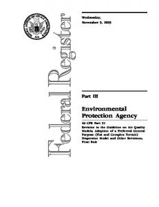
Anthropogenic VOC and NOx emissions are highest near urban areas. Figures 2-2 and 2-3 show the anthropogenic VOC and NO emissions by county across the United States. Notice that emissions levels correlate well with population levels, which are larger in the eastern third of the United States and near metropolitan areas. Along with anthropogenic emissions, the EPA also estimates annual biogenic emissions. Figure 2-4 shows that biogenic VOC emissions occur mostly in the forested regions of the United States (Southeast, Northeast, and West Coast regions). Biogenic VOC emissions include the highly reactive compound isoprene. Biogenic VOC emissions from forested and vegetative areas may impact urban ozone formation in some parts of the country. Biogenic NOx emissions levels are typically much lower than anthropogenic NOx emissions levels. 2-3
Figure 2-2. 1996 VOC emissions from anthropogenic sources by county (U.S. Environmental Protection Agency, 1997a).
Figure 2-3. 1996 NO emissions from anthropogenic sources by county (U.S. Environmental Protection Agency, 1997a).
2-4
Figure 2-4. 1996 VOC emissions from biogenic sources by county (U.S. Environmental Protection Agency, 1997a). 2.2
PARTICULATE MATTER
Particulate matter is the general term used for a mixture of solid particles and liquid droplets found in air. Numerous studies show association between morbidity/mortality and high PM concentrations. Studies also indicate that short-term exposure to acute PM concentrations can lead to long-term health effects. The negative health effects associated with high PM concentrations and the public’s desire for accurate air quality information has produced a need for PM forecasting programs that warn the public one or two days in advance of high PM concentrations. Since the EPA promulgated a new NAAQS for PM2.5 (PM less than 2.5 µm in diameter) in 1997 this guidance document has been updated to include information about forecasting PM2.5 concentrations. Much of the material summarized in the following sections was drawn from the PM2.5 Data Analysis Workbook (Main and Roberts, 2001), the PM criteria document (U.S. Environmental Protection Agency, 2001), Seinfeld and Pandis (1998), and documents referenced therein. 2.2.1
Basic Particulate Matter Chemistry
Particulate matter, unlike ozone, is not a specific chemical entity but is a mixture of particles of different sizes, shapes, compositions, and chemical, physical, and thermodynamic properties. Atmospheric PM2.5 results from primary fine particle emissions (emitted directly from sources) and emissions of gaseous compounds that form secondary aerosols. Secondary particles are formed from gases through chemical reactions in the atmosphere involving atmospheric oxygen (O2) and water vapor (H2O); reactive species such as ozone (O3); radicals such as the hydroxyl and nitrate radicals; and pollutants such as sulfur dioxide (SO2), nitrogen 2-5
oxides (NOx), ammonia (NH3), and volatile organic compounds (VOCs) from natural and anthropogenic sources. SO2 forms sulfates, NOx forms nitrates, NH3 forms ammonium compounds, and VOCs form organic carbon compounds. Some particles are liquid; some are solid. Others may contain a solid core surrounded by liquid. Atmospheric particles contain inorganic ions (e.g., nitrate, sulfate, sodium), metallic compounds, elemental carbon (EC), organic compounds, and crustal compounds (e.g., iron, calcium). Some atmospheric particles are hygroscopic and contain particle-bound water. The organic portion of PM is especially complex, containing hundreds of organic compounds. The particle formation process includes nucleation1 of particles from gases emitted from sources or formed in the atmosphere by chemical reactions, condensation of gases on existing particles, and coagulation of particles (Figure 2-5). Formation, transport, and removal rates are all a function of the particle size, chemical constituents of the particles, and meteorological processes (see Table 2-2).
Figure 2-5. Volume size distribution measured in traffic showing fine (including nuclei and accumulation modes) and coarse particle modes (Wilson and Suh, 1997). The geometric mean diameter by volume (DGV), equivalent to volume median diameter, and geometric standard deviation (σ2) are shown for each mode. Also shown are transformation and growth mechanisms (e.g., nucleation, condensation, and coagulation).
1
The formation of new particles.
2-6
Table 2-2. Summary of formation pathways, composition, sources, and atmospheric lifetimes of fine and coarse particulate matter (from Seinfeld and Pandis, 1998). Formation pathway
Composition
Sources
Atmospheric lifetime Travel distance
Fine Chemical reaction, nucleation, condensation, coagulation, cloud/fog processes Sulfate, nitrate, ammonium, hydrogen ion, elemental carbon, organics, water, metals (lead, cadmium, vanadium, nickel, copper, zinc, manganese, iron…) Combustion (coal, oil, gasoline, diesel, wood); gas-to-particle conversion of NOx, SOx, and VOCs; smelters, mills, etc. Days to weeks 100 to 1000+ km
Coarse Mechanical disruption, suspension of dust
Resuspended road dust; coal and oil flyash; crustal elements (silicon, aluminum, titanium, iron, usually as oxides); calcium carbonate, salt; pollen, mold, spores; plant and animal debris Resuspension of industrial soil and dust; suspension of soil (farming, mining, unpaved roads), biological sources, construction/demolition, ocean spray Minutes to days Generally < 100 km
The size of PM ranges from about tens of nanometers (nm) (which corresponds to molecular aggregates) to tens of microns (70 µm ≅ the size of a human hair) (see Figure 2-6). The smallest particles are generally more numerous, and the number distribution of particles generally peaks below 0.1 µm. The size range below 0.1 µm is also referred to as the ultrafine range. The largest particles (0.1-10 µm) are small in number but contain most of the PM volume (mass). The peak of the PM surface area distribution is always between the number and the volume peaks.
Particle diameter
Figure 2-6. Distribution of particle number, surface area, and volume or mass with respect to size (adapted from Husar, 1998). 2-7
2
Light Scattering and Absorption per Mass (m /g)
PM in the 0.1 to 1 micron size range has the longest residence time (days to weeks) because it neither settles nor coagulates quickly. Particles in this size range are the most efficient at penetrating deep into the lung. In addition, the light scattering efficiency per PM mass is highest at about 0.5 µm (see Figure 2-7). This is why, for example, 10 µg of fine particles scatter over 10 times more than 10 µg of coarse particles. Thus, PM2.5 is important to investigations of both human health and visibility impairment. Figure 2-7 also shows the absorption efficiency; there is little variation of the absorption efficiency as a function of particle size.
Figure 2-7. Relationship between light scattering, absorption, and particle diameter (Husar, 1998). Most secondary fine PM is formed from condensable vapors generated by chemical reactions of gas-phase precursors (i.e., vapors generated by chemical reactions condense to form particles). Secondary formation processes can result in either the formation of new particles or the addition of particulate material to pre-existing particles. Most of the sulfate and nitrate and a portion of the organic compounds in atmospheric particles are formed by chemical reactions in the atmosphere. Secondary aerosol formation depends on numerous factors including: •
The concentrations of precursors (which are a function of the proximity of emissions, wind speed, and mixing height).
•
The concentrations of other gaseous reactive species such as ozone, hydroxyl radical, peroxy radicals, or hydrogen peroxide (which are a function of solar radiation and temperature).
•
Atmospheric conditions, including solar radiation and relative humidity (RH).
•
The interactions of precursors and pre-existing particles within cloud or fog droplets or in the liquid film on solid particles. 2-8
As a result, it is considerably more difficult to relate ambient concentrations of secondary species to sources of precursor emissions than it is to identify the sources of primary particles. A diagram of these interactions is provided in Figure 2-8. Details about the chemical reactions can be found in Seinfeld and Pandis (1998), for example.
Sources
Emissions
PM Formation
PM Loss
Sample Collection
Chemical Processes Mechanical • Sea salt • Dust
Particles • NaCl • Crustal gases condense cloud/fog processes
Combustion • Motor vehicles • Industrial • Fires
Particles • Soot • Metals • OC Gases • NOx • SO2 • VOCs • NH3
Other gaseous • Biogenic • Anthropogenic
sedimentation (dry deposition) wet deposition condensation coagulation
Measurement Issues: • Inlet cut points • Vaporization of nitrate, H2O, VOCs • Adsorption of VOCs • Absorption of H2O
photochemical production cloud/fog processes
Gases • VOCs • NH3 • NOx
Meteorological Processes Winds Temperature Solar radiation Vertical mixing
Clouds, fog Temperature Relative humidity Solar radiation
Winds Precipitation
Temperature Relative humidity Winds
Figure 2-8. Sources of precursor gases and primary particles, PM formation processes, and removal mechanisms. Important meteorological measures are provided for each process. Sulfates Sulfates constitute about half of the PM2.5 in the eastern United States. Virtually all the ambient sulfate is secondary, formed within the atmosphere from SO2. About half of the conversion of SO2 to sulfate occurs in the gas phase through photochemical oxidation in the daytime. NOx and VOC emissions tend to enhance the photochemical oxidation rate. At least half of the SO2 oxidation takes place in cloud droplets as air molecules pass through convective clouds. Within clouds, the soluble pollutant gases, such as SO2, combine with water droplets and 2-9
rapidly oxidize to form sulfate. SO2-to-sulfate transformation rates peak in the summer due to enhanced summertime photochemical oxidation and SO2 oxidation in clouds. Conversion of SO2 to sulfate occurs at about 1% per hour in cloud-free air, but can convert to sulfate at 50% per hour in clouds and fog. Removal rates for SO2 (mostly by dry deposition) and sulfate (mostly by wet deposition) are about 2 to 3% per hour each. This gives sulfur (as SO2 and sulfate) an atmospheric residence time of from 1 to 5 days, depending on season, geography, and weather conditions. Nitrates Nitrates are a principal component of PM2.5 in the western United States and, like sulfates, are nearly all formed within the atmosphere from nitrogen oxide emissions. About onethird of anthropogenic NOx emissions in the United States are estimated to be removed by wet deposition. NO2 is converted to nitric acid by reaction with hydroxyl radicals during the day (oxidation). The reaction of hydroxyl radical with NO2 is 10 times faster than the oxidation of SO2. The peak daytime conversion rate of NO2 to nitric acid in the gas phase is about 10 to 50% per hour. During the nighttime, NO2 is converted into nitric acid by a series of reactions involving ozone and the nitrate radical. Nitric acid reacts with ammonia to form particulate ammonium nitrate. Thus, PM nitrate can be formed at night and during the day. Thermodynamically, nitrate formation is favored in cold, moist conditions. Thus, nitrate formation is enhanced in the winter compared to the summer. Organic and elemental carbon compounds Elemental carbon (EC), also called black carbon, is emitted directly into the atmosphere through combustion processes. Particulate organic carbon (OC) is both directly emitted and formed in secondary reactions. OC comprises a significant portion of the PM2.5 throughout the United States. Atmospheric reactions involving VOCs yield organic compounds with low vapor pressures at ambient temperature (i.e., the vapor or gas condenses to form a liquid). These reactions can occur in the gas phase, in fog or cloud droplets or in aqueous aerosols. Reaction products from the oxidation of VOCs also may nucleate to form new particles or condense on existing particles to form secondary organic PM. Both biogenic and anthropogenic sources contribute to primary and secondary organic particulate matter. Although the mechanisms and pathways for forming inorganic (i.e., sulfate, and nitrate) secondary particulate matter are fairly well known, those for forming secondary organic PM are not as well understood. Ozone and the hydroxyl radical are thought to be major contributing reactants. However, other radicals, including nitrate and organic radicals, are thought to contribute to secondary organic PM formation. Experimental studies of the production of secondary organic PM in ambient air have focused on the Los Angeles Basin. Evidence shows that secondary PM formation occurs during periods of photochemical ozone formation in Los Angeles and that as much as 70% of the organic carbon in ambient PM was secondary in origin during a smog episode in 1987 (see Turpin et al., 1991). Other experiments showed that 20 to 30% of the total organic carbon in fine PM in the Los Angeles airshed is secondary in origin on an annually averaged basis (Schauer et al., 1996). Thus, photochemical reactions are important to secondary organic carbon PM formation. 2-10
Another formation pathway is the adsorption of semi-volatile organic compounds (SVOCs, e.g., including polycyclic aromatic hydrocarbons)2 onto existing solid particles. This pathway can be driven by diurnal and seasonal temperature and humidity variations at any time of the year. Higher temperatures generally favor the gaseous phase of the SVOCs. 2.2.2
PM2.5 Emissions and Sources
The major constituents of atmospheric PM are sulfate, nitrate, ammonium, and hydrogen ions; particle-bound water; elemental carbon; a variety of organic compounds; and crustal material (see Table 2-3). These constituents can be primary or secondary. PM is called “primary” if it is in the same chemical form in which it was emitted into the atmosphere. PM is called “secondary” if it is formed by chemical reactions in the atmosphere. Primary fine particles are emitted from sources either directly as particles or as vapors that rapidly condense to form ultrafine particles (diameters < 0.1 micron) including: soot from diesel engines, a variety of organic compounds condensed from incomplete combustion or cooking, and metal compounds that condense from vapor formed during combustion or smelting. Table 2-3. Major PM2.5 components. Geological Material – suspended dust consists NaCl – salt is found in PM near sea coasts, mainly of oxides of aluminum, silicon, open playas, and after de-icing materials are calcium, titanium, iron, and other metal oxides. applied. The chloride ion can be replaced by nitrate as a result of reaction during long-range transport. Sulfate – results from conversion of SO2 gas to Organic Carbon (OC) – consists of hundreds sulfate-containing particles. of separate compounds containing mainly carbon, hydrogen, and oxygen. Nitrate – results from a reversible gas/particle Elemental Carbon (EC) – composed of equilibrium between ammonia, nitric acid, and carbon without much hydrocarbon or oxygen. particulate ammonium nitrate. EC is black, often called soot. Ammonium – ammonium bisulfate, sulfate, Liquid Water – soluble nitrates, sulfates, and nitrate are most common. ammonium, sodium, other inorganic ions, and some organic material absorb water vapor from the atmosphere. There are both anthropogenic and natural sources of PM2.5. Anthropogenic emissions that contribute to ambient PM2.5 concentrations include the following: •
Mobile sources. Gasoline- and diesel-fueled vehicles; resuspended road dust from vehicle activity on paved and unpaved roads; vehicle tire and brake wear; and off-road mobile sources such as trains, marine vessels, and farm machinery.
2
The phase in which an organic compound exists in the atmosphere is largely dependent on its vapor pressure. Nonvolatile compounds, such as polychlorinated biphenyls, exist almost exclusively on particulate matter (i.e., in the "particle phase"), whereas highly volatile compounds, such as small alkanes, remain in the gas phase. However, due to their intermediate volatility, the SVOCs partition between the gas and particle phases.
2-11
•
Stationary sources. Fuel combustion for electric utilities and industrial processes; fuel combustion for home heating; construction and demolition; metals, minerals, petrochemical, and wood products processing; mills and elevators used in agriculture; erosion from tilled lands; food cooking; and waste disposal and recycling.
Numerous natural sources also contribute primary and secondary particles to the atmosphere: •
Primary sources. Windblown dust from undisturbed land; sea spray; and plant and insect debris.
•
Secondary sources. Oxidation of naturally emitted biogenic hydrocarbons, such as terpenes, leads to formation of secondary organic PM2.5 and can accelerate the formation of inorganic secondary PM2.5, such as ammonium sulfate and ammonium nitrate.
•
Natural and man-made sources. Ammonia gas (precursor) and wood-burning particles (fuel wood burning and forest fires) are potentially important sources of PM2.5.
Since the precursor gases and PM2.5 are capable of long-range transport, it is often difficult to identify individual sources of PM2.5. It is especially difficult to distinguish contributions from natural and anthropogenic sources. The chemical composition of PM2.5 varies both geographically and seasonally (Figures 2-9 and 2-10). The composition may also vary with the magnitude of the PM2.5 mass concentrations. There are some relatively common characteristics across much of the United States, however, including: •
The crustal component is relatively small (