Empirical Evaluation of Data-based Density Estimation

Proceedings of the 2006 Winter Simulation Conference L. F. Perrone, F. P. Wieland, J. Liu, B. G. Lawson, D. M. Nicol, and R. M. Fujimoto, eds.

EMPIRICAL EVALUATION OF DATA-BASED DENSITY ESTIMATION

E. Jack Chen

W. David Kelton

BASF Corporation 333 Mount Hope Avenue Rockaway, New Jersey 07866, U.S.A.

Department of Quantitative Analysis and Operations Management University of Cincinnati Cincinnati, Ohio 45221, U.S.A.

ABSTRACT

data-based algorithm, i.e., the procedure can be embodied in a software package whose input is the data (X1 , . . . , Xn ) and whose output is the density estimate. Several different approaches have received extensive treatment; see Scott and Factor (1981) and the references in the paper. The most widely used density estimator is the histogram, a graphical estimate of the underlying probability density function and reveals all the essential distributional features of an output random variable analyzed by simulation, such as skewness and multimodality. Hence, a histogram is often used in the informal investigation of the properties of a given set of data. Given an origin g0 and a bin width w, the bins of the histogram are the intervals [g0 + mw, g0 + (m + 1)w] for positive and negative integers m. Suppose that we have any division of the real line into bins; then the histogram density estimator is

This paper discusses implementation of a sequential procedure to estimate the steady-state density of a stochastic process. The procedure computes sample densities at certain points and uses Lagrange interpolation to estimate the density f (x). Even though the proposed sequential procedure is a heuristic, it does have strong basis. Our empirical results show that the procedure gives density estimates that satisfy a pre-specified precision requirement. An experimental performance evaluation demonstrates the validity of using the procedure to estimate densities. 1

INTRODUCTION

Simulation studies have been used to investigate the characteristics of the system under study, for example the mean and the variance of certain system performance. The probability density function f gives a natural description of the distribution of the output random variable X produced by a simulation. The density function associated with X satisfies P(a < X < b) =

Z

1 (no. of Xi in same bin as x) . fˆh (x) = × n (width of bin containing x) Hence, to construct the histogram, we need to choose both an origin and a bin width. It is the bin width that, primarily, controls the amount of smoothing inherent in the procedure. Scott and Factor (1981) investigate the optimal bin width given a sample size. They point out that the optimal smoothing parameter can be computed if the true underlying sampling density f is known. A histogram can be constructed with a properly selected set of quantiles. It is known that for both independent and identically distributed (i.i.d.) and φ -mixing sequences sample quantiles will be asymptotically unbiased if certain conditions are satisfied; see Sen (1972). Intuitively, a stochastic process is φ -mixing if its distant future is essentially independent of its present and past (Billingsley 1999). In Section 2 we discuss some theoretical bases of density estimation in the context of simulation output analysis. In Section 3 we present our methodologies and the proposed procedure for density estimation. In Section 4 we show

b

f (x)dx for all a < b.

a

We investigate the performance of using the technique of Chen and Kelton (2006) to estimate the density of a simulation output random variable. Density estimation is the construction of an estimate of the density function from observed data. Silverman (1986, p. 5) points out that “density estimates are ideal for presentation of data to provide explanation and illustration of conclusions, since they are fairly easily comprehensible to non-mathematicians.” One approach to density estimation is parametric, assuming that the data are drawn from a known parametric family of distributions. Another approach is nonparametric, where less rigid assumptions are made about the distribution of the observed data. We consider the nonparameteric approach. Furthermore, the procedure is a

1-4244-0501-7/06/$20.00 ©2006 IEEE

333

Chen and Kelton 2.2 The Kernel Density Estimator

our empirical-experimental results of density estimation. In Section 5 we give concluding remarks. 2

To overcome the difficulties of ragged character, one can use a kernel function K, which satisfies the condition

THEORETICAL BASIS

Z

From the definition of a probability density, if the random variable X has density f , then f (x) = lim

h→0

∞

K(x)dx = 1.

−∞

1 P(x − h < X < x + h). 2h

For simplicity, function R the kernel RK usually is a symmetric R satisfying K(x)dx = 1, xK(x)dx = 0, and x2 K(x)dx = k2 6= 0; an example is the normal density. The kernel estimator with kernel K is defined by

2.1 The Histogram Density Estimator A natural estimator by histogram fˆh of the density is given by choosing a small number h (h = w/2) and setting

n

1 X K fˆk (x) = nh i=1

=

fˆh (x) 1 [no. of X1 , . . . , Xn falling in (x − h, x + h)]. 2nh

Ii =

x − Xi h



.

Silverman (1986, pp. 15-17) points out that “ fˆk will inherit all the continuity and differentiability properties of the kernel K, so that if K is the normal density function, then fˆk will be a smooth curve having derivatives of all orders.” However, the kernel method often underestimates the density at the boundary when the domain of the density being estimated is not the whole real line but an interval bounded on one or both sides; see Silverman (1986, p. 29). It can be shown that  Z  x−y 1 ˆ K f (y)dy; (1) E( fk (x)) = h h

Let p = P(|x − X| < h) and 



1 if |x − Xi | < h, 0 otherwise.

The estimator fˆh (x) is based on a transformation of the output sequence {Xi } to the sequence {Ii }, i = 1, 2, . . . , n: n

1 X fˆh (x) = Ii . 2nh i=1

Var( fˆk (x)) " Z  # 2 1 1 x−y 2 ˆ = K f (y)dy − E( fk (x)) n h2 h Z 1 f (x) K(y)2 dy, ≈ nh

For data that are i.i.d., the following properties of Ii are well known (Hogg and Craig 1995, pp. 116-117): E(Ii ) = p and Var(Ii ) = p(1 − p). Chen (2001) has developed a procedure to estimate proportion of simulation output sequences based on these properties. Since fˆh (x) is based on the mean of the random variable Ii , we can use any method developed for estimating the variance of the mean to estimate Var( fˆh (x)). Let I(·) denote the indicator function for the interval (x − h, x + h). It can be shown that E( fˆh (x)) =

1 2h

Z

and biash (x)

I (y) f (y)dy,

= E( fˆk (x) − f (x)) 1 2 00 = h f (x)k2 + higher-order terms in h. 2

See Silverman (1986, pp. 37-40) for details. The approximation of bias and variance indicates one of the fundamental difficulties of density estimation. To eliminate the bias, a small value of h should be used, but then the variance will become large. On the other hand, a large value of h will reduce the variance, but will increase the bias. Nevertheless, the ideal window width h should satisfy:

and Var( fˆh (x)) = p(1 − p)/(4nh2 ). Note that fˆh (x) has a binomial distribution. It follows from the definition that fˆh is not a continuous function, but has jumps at the points Xi ± h and has zero derivative everywhere else. This gives the estimate a somewhat ragged character.

lim h = 0, lim nh = ∞.

n→∞

334

n→∞

(2)

Chen and Kelton 3.1 Determine the Window Width

That is, h should converge to zero as the sample size increases but at a slower rate than n. Furthermore, smaller values of h will be appropriate for more rapidly fluctuating densities. R Let Jn = | fˆn − f |, where fˆn (x) = fn (x; X1 , . . . , Xn ) is a real-valued Borel measurable function of its arguments. Conditions (2) imply that there exists r ∈ R such that P(Jn ≥ 2 ε ) ≤ e−rnε for all ε ∈ (0, 1) and all n ≥ n f , where n f depends upon f and ε ; see Devroye and Gy¨orfi (1985). Since the shape of the true density is of most interest, a relevant criterion is the integrated mean squared error (IMSE) (Rosenblatt 1971) defined as Z Z IMSE = E[ fˆ(x) − f (x)]2 dx = E [ fˆ(x) − f (x)]2 dx.

Scott and Factor (1981) point out that “the great potential of nonparametric density estimators in data analysis is not being fully realized, primarily because of the practical difficulty associated with choosing the smoothing parameter given only data X1 , X2 , . . . , Xn .” Silverman (1986, p. 47) suggests that the window width of the kernel estimator be h = 0.9An−1/5 , where A = min(standard deviation, interquartile range/1.34).

There exists extensive research on the selection of an optimal kernel function to minimize the IMSE. Scott and Factor (1981) point out that many symmetric uni-modal kernel functions are nearly optimal. We use the Gaussian kernel in this paper. Moreover, it can be shown that the asymptotically optimal smoothing parameter is

For many purposes this will be an adequate choice of window width in terms of minimizing the IMSE. For others, it will be a good starting point for subsequent fine tuning. Let x p be the p sample quantile. In our procedure, we set

h = α (K)β ( f )n−1/5

Let x[1] and x[n] , respectively, denote the minimum and maximum of the initial n0 , 2n0 , or 3n0 observations, depending on the correlation of the output sequences. If (x[n] − x[1] )/(2h) < 25, then h will be halved. This adjustment is needed for distributions that have relatively large variance with a small range of the initial observations, so too large a window width. For example, if the estimated number of bins is 10, the procedure increases the number of bins to 20 and reduces the window width by half. We use the following strategy to determine the grid points. The are two categories of grids: main grids and auxiliary grids. Main grids are constructed based on the initial observations that “anchor” the grid of the simulationgenerated histogram, while auxiliary grids are extensions of main grids to ensure that the grids cover future observations. The number of main grid points is Gm = d(x[n] − x[1] )/(2h)e, and the number of auxiliary grid points is Ga = 2dδ Gm e, where 0 < δ < 1. The total number of grid points is thus G = Gm + Ga + 1. Let the beginning indices of the main grid point (i.e., the origin) be b = dδ Gm e + 1. The procedure sets gb+i = x[1] + 2ih, for i = 0, 1, . . . , Gm + Ga /2 − 1, and gb−i = x[1] − 2ih, for i = 1, 2, . . . , Ga /2 − 1. Grid point g1 is set to −∞ and gG is set to ∞. It is straightforward to compute the histogram density estimator. The array ni , i = 2, 3, . . . , G stores the number of observations between grid points gi−1 and gi , so the density of xi = (gi−1 + gi )/2 can be estimated by fˆ(xi ) = PG ni /(n(gi − gi−1 )), where n = i=2 ni is the total number of observations. To obtain the kernel estimator, the procedure needs to read through the output sequence again. In some sense, a simulation is just a function, which may be vector-valued or stochastic. The explicit form of this

A = min(standard error, (x0.75 − x0.25 )/2.68).

where

α (K) =

Z

1/5 Z −2/5 2 K(y) dy K(y)y dy 2

and

β(f) =

Z

00

2

f (x) dx

−1/5

.

With this choice, the IMSE decreases in proportion to n−4/5 ; see Scott and Factor (1981). 3

METHODOLOGIES

This section presents the methodologies we will use for our density estimation. A flow chart of the procedure is depicted in Figure 1. An imbedded pilot run is executed to set up the grid points. On each iteration, the algorithm operates as follows. The simulation outputs are funnelled into grids. The number of observations in each grid is updated as the observation is processed. The systematic samples are obtained through lag-l observations and are stored in a buffer. The initial value of l is 1. If lag-l 0 systematic samples appear to be dependent, then the lag l is doubled every other iteration and the process is repeated until the lag-l 0 systematic samples appear to be independent. The initial value of l 0 is 0 and will be updated each iteration by the following rule: “if l 0 < 3, then l 0 = l 0 + 1; else l 0 = 2.”

335

Chen and Kelton Start:Initialization

Collect observations: store lag l systmatic samples in buffer

Compute the no of observations in each grid when applicable

No

Buffers reach limit?

Determine the lag l' for test of independnece

Lag l' systematic samples appear to be IID?

No

Yes Reduce the no of systematic samples; double the lag l

Yes

Grid points have been established?

Yes No of iterations satisfied requirement?

Increase the no of replications

Yes

No

Compute the grid points

No

Yes Construct hitogram; compute density estimate

No

No

Density estimate meets precision requirements?

Yes

Deliver density estimate; Stop

Figure 1: Flow Chart of the Procedure 3.2 Determine the Sample Size

function is unknown. These plots (histograms) numerically characterize the distribution of the output sequence, even though we do not have an algebraic formula with which to characterize it. The procedure then computes the point density estimator via the histogram by (four-point) Lagrange interpolation (Knuth 1998). That is, for some k such that xk−1 < x ≤ xk , the x density point estimator can be computed as follows. Let wj =

4 Y

j0 =1, j0 6= j

The asymptotic validity of the density estimate is reached as the sample size or simulation run length gets large. However, in practical situations simulation experiments are restricted in time and it is not known in advance what is the required simulation run length for the estimator to become unbiased. Moreover, estimating the variance of the density estimator is needed to evaluate its precision. Therefore, a workable finite sample size must be determined dynamically for the precision required. We use an initial sample size of n0 = 600, which is somewhat arbitrary. If the underlying sequence is only slightly correlated and high precision is desired, a larger initial sample size should be used. For correlated sequences, the sample size n will be replaced with N = nl. Here l will be chosen sufficiently large so that systematic samples that are lag-l observations apart are statistically independent; see Chen and Kelton (2003). This is possible because we assume the underlying process satisfies the property that the autocorrelation approaches zero as the lag approaches infinity. Consequently, the final sample size N increases as the auto-correlation increases. In this procedure, we

x − xk+ j0 −3 , for j = 1, 2, 3, 4, xk+ j−3 − xk+ j0 −3

then fˆ(x) =

4 X

w j fˆ(xk+ j−3 ).

j=1

In two extreme cases, x1 < x ≤ x2 or xG−1 < x ≤ xG , linear interpolation will be used. Since the procedure uses interpolation to obtain point estimates, it eliminates the ragged character of the histogram. Hence, the density estimates for different points within the same bin can have different values.

336

Chen and Kelton as a point estimator of f (x). Assuming f¯(x) has a limiting normal distribution, by the central limit theorem a c.i. for f (x) using the i.i.d. fˆr (x)’s can be approximated using standard statistical procedures. That is, the ratio

use the von Neumann (1941) test of independence instead of the runs test. We can apply the von Neumann test of independence with a smaller sample size, but it has less power. Nevertheless, it serves the purpose well. Since we need to process the sequence again to obtain the kernel estimator, we re-compute the window width h with the final sample size N and the number of grid points with the new sample range. We only need to allocate main grids because the minimum and maximum are known. Furthermore, the sample error and the quantiles x0.25 and x0.75 will be estimated through the histogram constructed while calculating the natural estimator. That is, the variance is conservatively estimated by

T=

f¯(x) − f (x) √ S/ R

would have an approximate t distribution with R − 1 d.f. (degrees of freedom), where R 2 1 X ˆ ( fr (x) − f¯(x)) S = (R − 1) r=1 2

2 SH =

G X i=2

2 2 ¯ ¯ max((gi−1 − X(N)) , (g j − X(N)) )Pi .

PG

is the usual unbiased estimator of the variance of f (x). This would then lead to the 100(1 − α )% c.i., for f (x),

PN

¯ Note that N = nl = i=2 ni , X(N) = j=1 X j , and Pi = ni /N. To estimate the error, the IMSE is approximated by IMSE = 2

−1 Γ G X X

r=1 i=2

S f¯(x) ± tR−1,1−α /2 √ , R

(3)

where tR−1,1−α /2 is the 1− α /2 quantile for the t distribution with R − 1 d.f. (R ≥ 2). √ Let the half-width H be tR−1,1−α /2 S/ R. The final step in the procedure is to determine whether the c.i. meets the user’s half-width requirement, a maximum absolute halfwidth ε 0 or a maximum relative fraction γ of the magnitude of the final point density estimator f¯(x). If the relevant requirement H ≤ ε 0 or H ≤ γ | fˆ(x)| for the precision of the confidence interval is satisfied, then the procedure terminates, returns the point density estimator fˆ(x), and the c.i. with half-width H. If the precision requirement is not satisfied with R replications, then the procedure will increase the number of replications by one. This iterates until the pre-specified half-width is achieved.

[ fˆ(gi ) − f (gi )]2 h/Γ,

where Γ is the number of density estimates. The density of g1 and gG is not included in the calculation because they could be −∞ and ∞, respectively. Furthermore, if the true minimum (ω ) or the true maximum (Ω) are known, the values gi < ω or Ω < gi will not be included in the calculation. 3.3 Density Confidence Interval An approximate pointwise confidence interval (c.i.) for the density f (x) can be obtained using the binomial distribution from the histogram density estimate. The usual unbiased estimator of the variance of fˆh (x) is Sb2 = Var( fˆh (x)) = p(1 − p)/(4h2 N). This would then lead to the 100(1 − α )% c.i., for f (x),

4

EMPIRICAL EXPERIMENTS

We tested the proposed procedure with several i.i.d. and correlated sequences. In these experiments, we used R = 3 independent replications to construct c.i.’s. We constructed density c.i.’s at four points for each distribution. The confidence level 1 − α of the density c.i.— i.e., (3)—is set to 0.90. Moreover, the confidence level of the von Neumann test of independence is set to 0.90 as well. We tested the following independent sequences:

fˆh (x) ± z1−α /2 Sb , where z1−α /2 is the 1− α /2 quantile for the standard normal distribution. On the other hand, the distribution of fˆk (x) is unknown, hence, a c.i. cannot be constructed through one replication of fˆk (x). Let fˆr (x) denote the (histogram or kernel) estimator of f (x) in the rth replication. We use

•

Observations are i.i.d. from the tri-modal density f (x) = 2 2 2 1 1 √ (e−x /2 + e−(x−5) /8 + e−(x−10) /2 ). 2 3 2π

R

1Xˆ fr (x) f¯(x) = R r=1

337

Chen and Kelton •

Table 1: Coverage of 90% Confidence Density Estimators for the Tri-modal Distribution

Observations are i.i.d. from the exponential density f (x) =



e−x 0

if x ≥ 0 otherwise.

avg N 666 stdev N 119 x 0.5 5 7.5 10 f (x) 0.1226 0.0665 0.0363 0.1360 Histogram Estimator (0.001856, 0.000756) fˆ(x) 0.1193 0.0661 0.0373 0.1308 coverage 88.1% 91.5% 91.0% 84.3% avg γ 0.0515 0.0677 0.1007 0.0536 stdev γ 0.0389 0.0503 0.0749 0.0391 avg hw 0.0186 0.0150 0.0115 0.0192 stdev hw 0.0098 0.0078 0.0061 0.0106 Kernel Estimator (0.001207,0.000530) fˆ(x) 0.1155 0.0651 0.0392 0.1252 coverage 78.7% 88.7% 86.6% 63.3% avg γ 0.0621 0.0574 0.1003 0.0808 stdev γ 0.0395 0.0418 0.0731 0.0442 avg hw 0.0147 0.0118 0.0090 0.0151 stdev hw 0.0076 0.0060 0.0048 0.0117

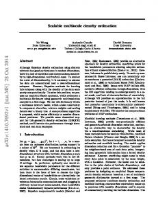
Tables 1 and 2 list the experimental results using the tri-modal and exponential distributions, respectively. Each design point was based on 1000 replications. The avg N row lists the average of the sample size of each independent run. The stdev N row lists the standard deviation of the sample size. The x row lists the point where we want to estimate density. The f (x) row lists the true density. The values after each the estimate method are the IMSE and the standard error of integrated squared error. The fˆ(x) row lists the grand mean of all density estimator from these 1000 replications. The coverage row lists the percentage of the c.i.’s that cover the true f (x). The avg γ row lists the average of the relative precision of the density estimators. Here, the relative precision is defined as γ = | fˆ(x) − f (x)|/ f (x). The stdev γ row lists the standard deviation of the relative precision of the density estimators. The avg hw row lists the average of the c.i. half-width. The stdev hw row lists the standard deviation of the c.i. half-width. As expected, the IMSE from the kernel estimator is better than from the histogram estimator. However, the kernel estimator requires more computation. In these experiments, no relative or absolute precisions were specified, so the half-width of the c.i. is the result of the default precision. In general, the histogram estimator has larger variance, so better c.i. coverage. However, the histogram estimators are biased high around the tail area. This is because the histogram estimators often result in a bounded distribution, i.e., the tail of the distribution is truncated. With α = 0.10, the independent sequences will fail the test of independence 10% of the times. The average sample sizes, 667, P∞ 666 and i , where n α are close to the theoretical value, i.e., 0 i=0 n0 = 600. Figures 2 and 3, respectively, show the empirical and true densities of the tri-modal and exponential distributions, generated from the first run of our experiments. The exponential distribution has a steep slope, so has a smaller window width h and has a more ragged empirical distribution curve. We tested the following correlated sequences: •

Table 2: Coverage of 90% Confidence Density Estimators for the Expon(1) Distribution avg N 667 stdev N 124 x 0.5 2.0 3.0 5.0 f (x) 0.6065 0.1353 0.0498 0.0067 Histogram Estimator (0.007100, 0.003581) fˆ(x) 0.6085 0.1359 0.0498 0.0088 coverage 90.4% 91.5% 90.0% 73.2% avg γ 0.0443 0.0950 0.1643 0.3612 stdev γ 0.0340 0.0699 0.1240 0.7372 avg hw 0.0885 0.0426 0.0263 0.0057 stdev hw 0.0491 0.0226 0.0137 0.0141 Kernel Estimator (0.003114, 0.001654) fˆ(x) 0.6116 0.1363 0.0502 0.0076 coverage 88.7% 90.4% 89.1% 86.5% 0.0316 0.0759 0.1304 0.4824 avg γ stdev γ 0.0248 0.0563 0.0989 2.9082 avg hw 0.0627 0.0339 0.0207 0.0100 stdev hw 0.0343 0.0182 0.0109 0.0572

−1 < ϕ < 1.

Observations are from the AR1 (first-order autoregressive) process:

•

Xi = µ + ϕ (Xi−1 − µ ) + εi for i = 1, 2, . . . ,

The AR1 process shares many characteristics observed in simulation output processes, including asymptotic firstand second-order stationarity, and autocorrelations that decline exponentially with increasing lag. If we make the additional assumption that the εi ’s are normally distributed, since we have already assumed that they are uncorrelated,

where E(εi ) = 0, E(εi ε j ) =



σ2 0

The εi ’s are commonly called error terms. Observations are from the M/M/1 queueing model.

if i = j , otherwise

338

Chen and Kelton for the kernel density estimate of x = 0.5, the c.i. coverages are above or close to the specified 90%. The kernel method encounters difficulty when estimating f (0.5) for the M/M/1 queueing process, because the value 0.5 is close to the discontinuity point 0. To deal with this difficulty, various adaptive methods have been proposed; see Silverman (1986, pp. 19-29). Figures 4 and 5, respectively, show the empirical distributions of the AR1 process with φ = 0.9 and the M/M/1 delay-in-queue process with ρ = 0.90, generated from the first run of our experiments. The theoretical steady-state distribution of this AR1 process and this M/M/1 queueing process are, respectively, N(0, 1/0.18) and 1 − 0.9e−0.1x , where x ≥ 0. Again, our experimental results show that these density estimates provide an excellent approximation of the underlying steady-state distributions. However, the kernel estimator over-smoothes the density around the discontinuity point.

Figure 2: Empirical Density of the Tri-modal Distribution

5

CONCLUSIONS

We have presented two algorithms for estimating the density f (x) of a stationary process. Since, to obtain the kernel estimator, the procedure needs to compute the histogram estimator, a prudent course is to choose any reasonable estimate based on these two estimates that are consistent with prior belief about the true sampling density. However, the histogram procedure is more suitable as a generic densityestimation procedure since it requires less computation, delivers a valid c.i., and has no difficulty estimating the density around a bounded tail or discontinuity point, though the IMSE is generally larger. Some density estimates require more observations than others before the asymptotics necessary for density estimates become valid. Our algorithm works well in determining the required simulation run length for the asymptotic approximation to become valid. The results from our empirical experiments show that the procedure is excellent in achieving the pre-specified accuracy. Our proposed histogramapproximation algorithm computes quantiles only at grid points and uses Lagrange interpolation to estimate the density at certain points. The algorithm also generates an empirical distribution (histogram) of the output sequence, which can provide insights into the underlying stochastic process. Our approach has the desirable properties that it is a sequential procedure and it does not require users to have a priori knowledge of values that the data might assume. This allows the user to apply this method without having to execute a separate pilot run to determine the range of values to be expected, or guess and risk having to re-run the simulation. The main advantage of our approach is that by using a straightforward test of independence to determine the simulation run length and obtain quantiles at grid points,

Figure 3: Empirical Density of the Exponential Distribution

they will now be independent as well, i.e., the εi ’s are i.i.d. N (0, 1), where N (µ , σ 2 ) denotes a normal distribution with mean µ and variance σ 2 . It can be shown that X has asymptotically a N (0, 1−1ϕ 2 ) distribution, and the steadystate variance constant of the AR(1) process is 1/(1 − ϕ )2 . We set ϕ to 0.90 and set µ to zero for this experiment. In order to eliminate the initial bias, X0 is set to a random variate drawn from the steady-state distribution. Table 3 lists the experimental results of the AR1 process. The c.i. coverage of these four design points are around the specified 90% confidence level for both estimators. The simulation run length generally increases as the correlation coefficient ϕ of the AR(1) process increases. The run length of the AR1 process with ϕ = 0.9 is much larger than independent sequences and consequently much smaller IMSE. The waiting-time density of the stationary M/M/1 delay in queue is f (x) = (ν − λ ) λν e−(ν −λ )x for x ≥ 0 and is discontinuous at x = 0, where λ is the arrival rate and ν is the service rate. Summary of our experimental results of the M/M/1 delay-in-queue process is in Table 4. Except

339

Chen and Kelton we can apply classical statistical techniques directly and do not require more advanced statistical theory, thus making it easy to understand, and simple to implement. Table 3: Coverage of 90% Confidence Density Estimators for the AR1(0.9) Process avg N 20965 stdev N 3836 x -0.5 0.0 1.0 2.0 f (x) 0.1698 0.1739 0.1581 0.1189 Histogram Estimator (0.000221, 0.000133) fˆ(x) 0.1697 0.1737 0.1579 0.1190 coverage 89.6% 89.7% 89.1% 90.4% avg γ 0.0138 0.0132 0.0147 0.0192 stdev γ 0.0107 0.0105 0.0111 0.0148 avg hw 0.0075 0.0076 0.0077 0.0074 stdev hw 0.0041 0.0042 0.0041 0.0038 Kernel Estimator (0.000209, 0.000128) fˆ(x) 0.1696 0.1737 0.1578 0.1189 coverage 88.7% 88.9% 90.7% 90.4% 0.0142 0.0133 0.0151 0.0190 avg γ stdev γ 0.0107 0.0103 0.0110 0.0142 avg hw 0.0074 0.0076 0.0077 0.0074 stdev hw 0.0041 0.0042 0.0041 0.0038

Figure 4: Empirical Density of the AR1 Process

Table 4: Coverage of 90% Confidence Density Estimators for the MM1(0.9) Process avg N 418496 stdev N 92729 x 0.5 2.5 5.0 10.0 f (x) 0.0856 0.0701 0.0546 0.0331 Histogram Estimator (0.000021, 0.000020) ˆ f (x) 0.0833 0.0704 0.0547 0.0331 coverage 85.0% 90.8% 92.6% 91.2% avg γ 0.0295 0.0102 0.0082 0.0093 stdev γ 0.0232 0.0083 0.0064 0.0070 avg hw 0.0050 0.0023 0.0015 0.0010 stdev hw 0.0034 0.0013 0.0008 0.0006 Kernel Estimator (0.0000021, 0.000017) fˆ(x) 0.1657 0.0701 0.05460 0.0331 coverage 0.0% 91.2% 91.3% 90.4% avg γ 0.9355 0.0086 0.0082 0.0096 stdev γ 0.0291 0.0063 0.0063 0.0076 avg hw 0.0066 0.0020 0.0015 0.0010 stdev hw 0.0037 0.0011 0.0008 0.0006

Figure 5: Empirical Density of the M/M/1 Process

Chen, E. J. 2001. Proportion estimation of correlated sequences. Simulation 76 (5): 273-276, 301-304. Chen, E. J., and W. D. Kelton. 2003. Determining simulation run length with the runs test. Simulation Modelling Practice and Theory 11 (3-4): 237-250. Chen, E. J., and W. D. Kelton. 2006. Estimating steadystate distributions via simulation-generated histograms. Computer and Operations Research. To Appear. Devroye, L., and L. Gy¨orfi. 1985. Nonparametric density estimation: the L1 view. New York: John Wiley & Sons. Hogg, R. V., and A. T. Craig. 1995. Introduction to mathematical statistics. Fifth Edition. Englewood Cliffs, New Jersey: Prentice Hall. Knuth, D. E. 1998. The art of computer programming. Vol. 2. 3rd ed. Reading, Mass.: Addison-Wesley. Rosenblatt, M. 1971. Curve estimates. Annals of Mathematical Statistics 42:1815-1842.

REFERENCES Billingsley, P. 1999. Convergence of probability measures. 2nd ed. New York: John Wiley & Sons.

340

Chen and Kelton Scott, D. W., and L. E. Factor. 1981. Monte carlo study of three data-based nonparametric probability density estimators. Journal of the American Statistical Association 76 (373):9–15. Sen, P. K. 1972. On the Bahadur representation of sample quantiles for sequences of φ -mixing random variables. Journal of Multivariate Analysis 2 (1):77–95. Silverman, B. W. 1986. Density estimation for statistics and data analysis. New York: Chapman and Hall. von Neumann, J. 1941. Distribution of the ratio of the mean square successive difference and the variance. Annals of Mathematical Statistics 12:367–395. AUTHOR BIOGRAPHIES E. JACK CHEN is a Senior Staff Specialist with BASF Corporation. He received a Ph.D. from the University of Cincinnati. His research interests are in the area of computer simulation. His email address is . W. DAVID KELTON is a Professor in the Department of Quantitative Analysis and Operations Management at the University of Cincinnati. He received a B.A. in mathematics from the University of Wisconsin-Madison, an M.S. in mathematics from Ohio University, and M.S. and Ph.D. degrees in industrial engineering from Wisconsin. His research interests and publications are in the probabilistic and statistical aspects of simulation, applications of simulation, and stochastic models. Currently, he serves as Editor-inChief of the INFORMS Journal on Computing, and has been Simulation Area Editor for Operations Research, the INFORMS Journal on Computing, and IIE Transactions, as well as Associate Editor for Operations Research, the Journal of Manufacturing Systems, and Simulation. From 1991 to 1999 he was the INFORMS co-representative to the Winter Simulation Conference Board of Directors and was Board Chair for 1998. In 1987 he was Program Chair for the WSC, and in 1991 was General Chair. His email and web addresses are and .

341