Multi-dimensional Density Estimation David W. Scott a,∗,1, Stephan R. Sain b,2 a Department b Department
of Statistics, Rice University, Houston, TX 77251-1892, USA of Mathematics, University of Colorado at Denver, Denver, CO 80217-3364 USA
Abstract Modern data analysis requires a number of tools to undercover hidden structure. For initial exploration of data, animated scatter diagrams and nonparametric density estimation in many forms and varieties are the techniques of choice. This article focuses on the application of histograms and nonparametric kernel methods to explore data. The details of theory, computation, visualization, and presentation are all described. Key words: Averaged shifted histograms, Contours, Cross-validation, Curse of dimensionality, Exploratory data analysis, Frequency polygons, Histograms, Kernel estimators, Mixture models, Visualization PACS: 62-07, 62G07
1
Introduction
Statistical practice requires an array of techniques and a willingness to go beyond simple univariate methodologies. Many experimental scientists today are still unaware of the power of multivariate statistical algorithms, preferring ∗ Corresponding author. Email addresses:
[email protected],
[email protected] (Stephan R. Sain). 1 This research was supported in part by the National Science Foundation grants NSF EIA-9983459 (digital government) and DMS 02-04723 (non-parametric methodology). 2 This research was supported in part through the Geophysical Statistics Project at the National Center for Atmospheric Research under National Science Foundation grant DMS 9815344.
Preprint submitted to Elsevier Science
31 August 2004
the intuition of holding all variables fixed, save one. Likewise, many statisticians prefer the familiarity of parametric statistical techniques and forgo exploratory methodologies. In this chapter, the use of density estimation for data exploration is described in practice with some theoretical justification. Visualization is an important component of data exploration, and examples of density surfaces beyond two dimensions will be described. We generally consider the analysis of a d-variate random sample (x1 , . . . , xn ) from an unknown density function, f (x), where x ∈ 0 and ki=1 pi = 1. The components of the mixture, {gi , i = 1, . . . , k}, are themselves densities and are parameterized by θ i which may be vector valued. Often, the gi are taken to be multivariate normal, in which case θ i = {µi , Σi }. Mixture models are often motivated by heterogeneity or the presence of distinct subpopulations in observed data. For example, one of the earliest applications of a mixture model (Pearson, 1894; see also McLachlan and Peel, 2000) used a two-component mixture to model the distribution of the ratio between measurements of forehead and body length on crabs. This simple mixture was effective at modeling the skewness in the distribution and it was hypothesized that the two-component structure was related to the possibility of this particular population of crabs evolving into two new subspecies. The notion that each component of a mixture is representative of a particular subpopulation in the data has led to the extensive use of mixtures in the context of clustering and discriminant analysis. See, for example, the reviews by Fraley and Raftery (2002) and McLachlan and Peel (2000). It was also the motivation for the development of the multivariate outlier test of Wang et al. (1997) and Sain et al. (1999), who were interested in distinguishing nuclear tests from a background population consisting of different types of earthquakes, mining blasts, and other causes. Often, a mixture model fit to data will have more components than can be identified with the distinct groups present in the data. This is due to the flexibility of mixture models to represent features in the density that are not well-modeled by a single component. Marron and Wand (1992), for example, give a wide variety of univariate densities (skewed, multimodel, e.g.) that are constructed from normal mixtures. It is precisely this flexibility that makes 24
mixture models attractive for general density estimation and exploratory analysis. When the number of components in a mixture is pre-specified based on some a priori knowledge about the nature of the subpopulations in the data, mixtures can be considered a type of parametric model. However, if this restriction on the number of components is removed, mixtures behave in nonparametric fashion. The number of components acts something like a smoothing parameter. Smaller numbers of components will behave more like parametric models and can lead to specification bias. Greater flexibility can be obtained by letting the number of components grow, although too many components can lead to overfitting and excessive variation. A parametric model is at one end of this spectrum, and a kernel estimator is at the other end. For example, a kernel estimator with a normal kernel can be simply considered a mixture model with weights taken to be 1/n and component means fixed at the data points. 4.1 Fitting Mixture Models While mixture models have a long history, fitting mixture models was problematic until the advent of the expectation-maximization (EM) algorithm of Dempster, Laird, and Rubin (1977). Framing mixture models as a missing data problem has made parameter estimation much easier, and maximum likelihood via the EM algorithm has dominated the literature on fitting mixture models. However, Scott (2001) has also had considerable success using the L2 E method, which performs well even if the assumed number of components, k, is too small. The missing data framework assumes that each random vector Xi generating from the density (21) is accompanied by a categorical random variable Zi where Zi indicates the component from which Xi comes. In other words, Zi is a single-trial multinomial with cell probabilities given by the mixing proportions {pi }. Then, the density of Xi given Zi is gi in (21). It is precisely the realized values of the Zi that are typically considered missing when fitting mixture models, although it is possible to also consider missing components in the Xi as well. For a fixed number of components, the EM algorithm is iterative in nature and has two steps in each iteration. The algorithm starts with initial parameter estimates. Often, computing these initial parameter estimates involves some sort of clustering of the data, such as a simple hierarchical approach. The first step at each iteration is the expectation step which involves prediction and effectively replaces the missing values with their conditional expectation given the data and the current parameter estimates. The next step, the max25
imization step, involves recomputing the estimates using both complete data and the predictions from the expectation step. For normal mixtures missing only the realized component labels zi , this involves computing in the expectation step ˆ 0) ˆ 0j , Σ pˆ0j fj (xi ; µ j wij = Pk 0 ˆ0 0 ˆ j , Σj ) ˆj fj (xi ; µ j=1 p
(22)
ˆ 0 are the curˆ 0j , and Σ for i = 1, . . . , n and j = 1, . . . , k and where pˆ0j , µ j rent parameter estimates. The maximization step then updates the sufficient statistics
Tj1 =
n X
wij ;
Tj2 =
n X
wij xi ;
Tj3 =
wij xi x0i
i=1
i=1
i=1
n X
for j = 1, . . . , k to yield the new parameter estimates pˆ1j = Tj1 /n ;
ˆ 1j = Tj2 /Tj1 ; µ
ˆ 1 = (Tj3 − Tj2T0 /Tj1 )/Tj1 Σ j j2
for j = 1, . . . , k. The process cycles between these two steps until some sort of convergence is obtained. The theory concerning the EM algorithm suggests that the likelihood is increased at each iteration. Hence, at convergence, a local maximum in the likelihood has been found. A great deal of effort has been put forth to determine a data-based choice of the number of components in mixture models and many of these are summarized in McLachlan and Peel (2000). Traditional likelihood ratio tests have been examined but a breakdown in the regularity conditions have made implementation difficult. Bootstrapping and Bayesian approaches have also been studied. Other criterion such as Akaike’s information criterion (AIC) have been put forth and studied in some detail. In many situations, however, it has been found that AIC tends to choose too many components. There is some criticism of the theoretical justification for AIC, since it violates the same regularity conditions as the likelihood ratio test. An alternative information criterion is the Bayesian information criterion (BIC) given by BIC = −2` + d log n where ` is the maximized log-likelihood, d is the number of parameters in the model, and n is the sample size. While there are some regularity conditions for BIC that do not hold for mixture models, there is much empirical evidence that supports its use. For example, Roeder and Wasserman (1997) show that 26
2 0
log(precipitation)
−4
−2
2 0
log(precipitation)
−2 −4
−60
−40
−20
0
20
−60
temperature
−40
−20
0
20
temperature
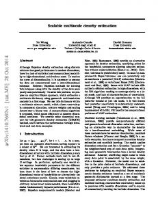
Fig. 10. Example using climate data. The best BIC model uses six components and these components are represented by ellipses in the left frame. The right frame shows a contour plot of the resulting density estimate.
when a normal mixture model is used as a nonparametric density estimate, the density estimate that uses the BIC choice of the number of components is consistent. Other sophisticated procedures for choosing the number of components in mixture models have also been explored. For example, Priebe and Marchette (1991; 1993) and Priebe (1994) discuss what the authors’ refer to as “adaptive mixtures” that incorporate the ideas behind both kernel estimators and mixture models and that use a data-based method for adding new terms to a mixture. The adaptive mixture approach can at times overfit data and Solka et al. (1998) combine adaptive mixtures with a pruning step to yield more parsimonious models. These methods have also been shown, both theoretically and through simulation and example, to be effective at determining the underlying structure in the data.
4.2 An Example
Figures 10 and 11 show an example of an application of a mixture model using bivariate data consisting of twenty-year averages of temperature and precipitation measured globally on a 5◦ grid (Covey et al., 2003; Wigely, 2003). An initial scatterplot of the measurements shows clearly the presence of multiple groupings in the data. It is hypothesized that this multimodality can be attributed to climatic effects as well as latitude and land masses across the globe. A sequence of multivariate normal mixture models was fit to the data using 27
Fig. 11. An image plot displaying the results of the clustering based on the mixture estimate. The effects of land masses and latitude are clearly present in the clusters.
various numbers of components. BIC suggested a six component model. The ellipses in the left frame of Figure 10 indicate location and orientation of the individual components while the right frame shows the contours of the resulting density overlaid on the data. It seems clear from the contour plot that some components are present to model non-normal behavior in the density. However, Figure 11 shows the result of classifying each observation as coming from one of the six components. This is done by examining the posterior probabilities as given by the wij in (22) at the end of the EM iterations. The groupings in the data do appear to follow latitude lines as well as the land masses across the globe.
5
Visualization of Densities
The power of nonparametric curve estimation is in the representation of multivariate relationships. While univariate density estimates are certainly useful, the visualization of densities in two, three, and four dimensions offers greater potential in an exploratory context for feature discovery. Visualization techniques are described here. We examine the zip code data described by Le Cun et al. (1990). Handwritten digits scanned from USPS mail were normalized into 16 × 16 grayscale images. Training and testing data (available at the U.C. Irvine data repository) were combined into one data set, and the digits 1, 3, 7, and 8 were extracted for analysis here (1269, 824, 792, and 708 cases, respectively). We selected these digits to have examples of straight lines (1 and 7) as well as curved digits (3 and 8). In Figure 12, some examples of the digits together with summary statistics are displayed. Typical error rates observed classifying these data are high, in the 2.5% range. 28
Fig. 12. (Left) Mean, standard deviation, and examples of zip code digits 1, 3, 7, and 8. (Right) LDA subspace of zip code digits 1 (×), 3 (•), 7 (+), and 8 (O). 1
7 1
1
3 8 7 7
8
3 3
8
Fig. 13. ASH’s for each of the 4 digits for the 1st, 2nd, and 3rd LDA variable (L-R).
To analyze and visualize these data, we computed the Fisher linear discriminant analysis (LDA) subspace. We sphered the data using a pooled covariance estimate, and computed the LDA subspace as the three-dimensional span of the four group means. The right frame of Figure 12 displays a frame from xgobi (Swayne, Cook, and Buja, 1991) and shows that the four groups are reasonably well-defined and separated in the LDA variable space. If we examine averaged shifted histograms of each digit for each of the three LDA variables separately, we observe that the first LDA variable separates out digit 1 from the others; see the left frame Figure 13. In the middle frame, the second LDA variable separates digit 7 from digits 3 and 8. Finally, in the right frame, the third LDA variable almost completely separates digits 3 and 8 from each other (but not from the others). We can obtain a less fragmented view of the feature space by looking at pairs of the LDA variables. In Figures 14 and 15, averaged shifted histograms for each digit were computed separately and are plotted. Contours for each ASH were drawn at 10 equally-spaced levels. The left frame in Figure 14 reinforces the notion that the first two LDA variables isolate digits 1 and 7. Digits 3 and 8 are separated by the first and third LDA variables in the right frame of Figure 14; recall that digit 7 can be isolated using the second LDA variables. Interestingly, in Figure 15, all four digits are reasonably separated by the 29
3
8
3 8
1
8
1
1
8
7
1
7 3
7
7
3
Fig. 14. Bivariate ASH’s of the 4 digits using LDA variables (v1 , v2 ) (left) and (v1 , v3 ) (right) .
8 8
8
7 3
1 7
1
1
3
7
3
Fig. 15. ASH’s for LDA variables (v2 , v3 ).
second and third LDA variables alone. We also show a perspective plot of these ASH densities. (The perspective plot in Figure 14 does not display the full 100 × 100 mesh at this reduced size for clarity and to avoid overplotting the lines.) Visualization of univariate and bivariate densities has become a fairly routine task in most modern statistical software packages. The figures in this chapter were generated using the Splus package on a Sun under the Solaris operating system. The ASH software is available for download at the ftp software link at author’s homepage www.stat.rice.edu/∼scottdw. The ASH software contains separate routines for the univariate and bivariate cases. Visualization of the ash1 and ash2 estimates was accomplished using the built-in Splus functions contour and persp. A separate function, ashn, is also included in the ASH package. The ashn function not only computes the ASH for dimensions 3 ≤ d ≤ 6, but it also provides the capability to visualize arbitrary three-dimensional contours of a level set of any four-dimensional surface. In particular, if fmax is the maximum value of an ASH estimate, fˆ(x, y, z), and α takes values in the interval (0, 1), 30
then the α-th contour or level set is the surface Cα = {(x, y, z) : fˆ(x, y, z) = α fmax } . The mode of the density corresponds to the choice α = 1. The ashn function can compute the fraction of data within any specified α-contour. Some simple examples of Cα contours may be given for normal data. If the covariance matrix Σ = Id , then contours are spheres centered at µ: 2 +(y−µ )2 +(z−µ )2 ) 2 3
Cα = {(x, y, z) : e−0.5((x−µ1 )
= α}
or Cα = {(x, y, z) : (x − µ1 )2 + (y − µ2 )2 + (z − µ3 )2 = −2 log α}. For a general covariance matrix, the levels sets are the ellipses Cα = {(x, y, z) : (x − µ)0 Σ−1 (x − µ) = −2 log α}. With a nonparametric density, the contours do not follow a simple parametric form and must be estimated from a matrix of values, usually on a regular three-dimensional mesh. This mesh is linearly interpolated, resulting in a large number of triangular mesh elements that are appropriately sorted and plotted in perspective. Since the triangular elements are contiguous, the resulting plot depicts a smooth contour surface. This algorithm is called marching cubes (Lorensen and Cline, 1987). In Figure 16, a trivariate ASH is depicted for the data corresponding to digits 3, 7, and 8. (The digit 1 is well-separated and those data are omitted here.) The triweight kernel was selected with m = 7 shifts for each dimension. The contours shown correspond to the values α = 0.02, 0.1, 0.2, 0.35, 0.5, 0.7, and 0.9. The ashn function also permits an ASH to be computed for each of the digits separated and plotted in one frame. For these data, the result is very similar to the surfaces shown in Figure 16. This figure can be improved further by using stereo to provide depth of field, or through animation and rotation. The ashn software has an option to output this static figure in the so-called QUAD format used by the geomview visualization package from the previous NSF Geometry Center in Minneapolis. This software is still available from www.geomview.org and runs on SGI, Sun, and Linux platforms (Geomview, 1998). 5.1 Higher Dimensions Scott (1992) describes extensions of the three-dimensional visualization idea to four dimensions or more. Here we consider just four-dimensional data, 31
z
x y
Fig. 16. Trivariate ASH of LDA variables (v1 , v2 , v3 ) and digits 3, 7, and 8. The digit labels were not used in this plot. The digit 7 is in the left cluster; the digit 8 in the top cluster; and the digit 3 in the lower right cluster.
(x, y, z, t). The α-th contour is defined as above as Cα = {(x, y, z, t) : fˆ(x, y, z, t) = α fmax } . Since only a 3-dimensional field may be visualized, we propose to depict slices of the four-dimensional density. Choose a sequence of values of the fourth variable, t1 < t2 < · · · < tm , and visualize the sequence of slices Cα (k) = {(x, y, z) : fˆ(x, y, z, t = tk ) = α fmax }
for k = 1, . . . , m .
With practice, observing an animated view of this sequence of contours reveals the four-dimensional structure of the five-dimensional density surface. An important detail is that fmax is not recomputed for each slice, but remains the constant value of maximum of the entire estimate fˆ(x, y, z, t). A possible alternative is viewing the conditional density, fˆ(x, y, z|t = tk ); however, the renormalization destroys the perception of being in the low-density or tails of the distribution. To make this idea more concrete, let us revisit the trivariate ASH depicted in Figure 16. This ASH was computed on a 75 × 75 × 75 mesh. We propose ˆ y, z) to examine the as an alternative visualization of this ASH estimate f(x, sequence of slices Cα (k) = {(x, y, z) : fˆ(x, y, z = zk )} 32
for k = 1, . . . , 75 .
6
10
14
18
22
26
30
34
38
42
46
50
54
58
62
Fig. 17. A sequence of slices of the three-dimensional ASH of the digits 3, 7, and 8 depicted in Figure 16. The z-bin number is shown in each frame from the original 75 bins.
In Figure 17, we display a subset of this sequence of slices of the trivariate ASH estimate. For bins numbered less than 20, the digit 3 is solely represented. For bins between 22 and 38, the digit 7 is represented in the lower half of each frame. Finally, for bins between 42 and 62, the digit 8 is solely represented. We postpone an actual example of this slicing technique for 4-dimensional data, since space is limited. Examples may be found in the color plates of Scott (1992). The extension to five-dimensional data is straightforward. The ashn package can visualize slices such as the contours Cα (k, `) = {(x, y, z) : fˆ(x, y, z, t = tk , s = s` ) = α fˆmax } . Scott (1986) presented such a visualization of a five-dimensional dataset using an array of ASH slices on the competition data exposition at the Joint Statistical Meetings in 1986. 5.2 Curse of Dimensionality As noted by many authors, kernel methods suffer from increased bias as the dimension increases. We believe the direct estimation of the full density by kernel methods is feasible in as many as six dimensions. However, this does not mean that kernel methods are not useful in dimensions beyond six. Indeed, for purposes such as statistical discrimination, kernel 33
methods are powerful tools in dozens of dimensions. The reasons are somewhat subtle. Scott (1992) argued that if the smoothing parameter is very small, then comparing two kernel estimates at the same point x is essentially determined by the closest point in the training sample. It is well-known that the nearest-neighbor classification rule asymptotically achieves half of the optimal Bayesian misclassification rate. At the other extreme, if the smoothing parameter is very large, then comparing two kernel estimates at the same point x is essentially determined by which sample mean is closer for the two training samples. This is exactly what Fisher’s LDA rule does in the LDA variable space. Thus, at the extremes, kernel density discriminate analysis mimics two well-known and successful algorithms. Thus there exist a number of choices for the smoothing parameter between the extremes that produce superior discriminate rules. What is the explanation for the good performance for discrimination and the poor performance for density estimation? Friedman (1997) argued that the optimal smoothing parameter for kernel discrimination was much larger than for optimal density estimation. In retrospect, this result is not surprising. But it emphasizes how suboptimal density estimation can be useful for exploratory purposes and in special applications of nonparametric estimation.
6
Discussion
There are a number of useful references for the reader interested in pursuing these ideas and others not touched upon in this chapter. Early reviews of nonparametric estimators include Wegman (1972a, b) and Tarter and Kronmal (1976). General overviews of kernel methods and other nonparametric estimators include Tapia and Thompson (1978), Silverman (1986), H¨ardle (1990), Scott (1992), Wand and Jones (1995), Fan and Gijbels (1996), Simonoff (1996), Bowman and Azzalini (1997), Eubank (1999), Schimek(2000), and Devroye and Lugosi (2001). Scott (1992) and Wegman and Luo (2002) discuss a number of issues with the visualization of multivariate densities. Classic books of general interest in visualization include Wegman and DePriest (1986), Cleveland (1993), Wolff and Yaeger (1993), and Wainer (1997). Applications of nonparametric density estimation are nearly as varied as the field of statistics itself. Research challenges that remain include handling massive datasets and flexible modeling of high-dimensional data. Mixture and semiparametric models hold much promise in this direction. 34
References [1] Abramson, I.: On Bandwidth Variation in Kernel Estimates -A Square Root Law. The Annals of Statistics, 10, 1217–1223 (1982) [2] Banfield, J.D. and Raftery, A.E.: Model-based Gaussian and non-Gaussian clustering. Biometrics, 49, 803–821 (1993) [3] Bowman, A.W.: An Alternative Method of Cross-Validation for the Smoothing of Density Estimates. Biometrika, 71, 353–360 (1984). [4] Bowman, A.W., and Azzalini, A.: Applied Smoothing Techniques for Data Analysis: the Kernel Approach with S-Plus Illustrations. Oxford University Press, Oxford: (1997) [5] Breiman, L., Meisel, W., and Purcell, E.: Variable kernel estimates of multivariate densities. Technometrics, 19, 353–360 (1977) [6] Chaudhuri, P. and Marron, J.S.: SiZer for exploration of structures in curves. Journal of the American Statistical Association, 94, 807–823 (1999) [7] Cleveland, W.S.: Visualizing Data. Hobart Press, Summit, NJ (1993) [8] Covey, C., AchutaRao, K.M., Cubasch, U., Jones, P.D., Lambert, S.J., Mann. M.E., Phillips, T.J. and Taylor, K.E.: An overview of results from the Coupled Model Intercomparison Project (CMIP). Global and Planetary Change, 37, 103–133 (2003) [9] Dempster, A.P., Laird, N.M., and Rubin, D.B.: Maximum likelihood for incomplete data vi the EM algorithm (with discussion). Journal of the Royal Statistical Society, Ser. B, 39, 1–38 (1977) [10] Devroye, L. and Lugosi, T.: Variable kernel estimates: On the impossibility of tuning the parameters. In: Gine, E. and Mason, D. (ed) HighDimensional Probability. Springer, New York (2000) [11] Devroye, L. and Lugosi, T.: Combinatorial methods in density estimation. Springer-Verlag, Berlin (2001) [12] Donoho, D.L., Johnstone, I.M., Kerkyacharian, G., and Picard, D.: Density estimation by wavelet thresholding. The Annals of Statistics, 24, 508– 539 (1996) [13] Duin, R.P.W.: On the choice of smoothing parameters for Parzen estimators of probability density functions. IEEE Transactions on Computers, 25, 1175–1178 (1976) [14] Eilers, P.H.C. and Marx, B.D.: Flexible smoothing with B-splines and penalties. Statistical Science, 11, 89–102 (1996) [15] Eubank, R.L.: Nonparametric Regression and Spline Smoothing. Marcel Dekker, New York (1999) [16] Fan, J. and Gijbels, I.: Local Polynomial Modelling and Its Applications. Chapman and Hall, London (1996) [17] Fisher, R.A.: Statistical Methods for Research Workers, Fourth Edition. Oliver and Boyd, Edinburgh (1932) [18] Fraley, C. and Raftery, A.E.: Model-based clustering, discriminant analysis, and density estimation. Journal of the American Statistical Association, 97, 611–631 (2002) 35
[19] Friedman, J.H.: On Bias, Variance, 0/1-Loss, and the Curse-of-Dimensionality. Data Mining and Knowledge Discovery, 1, 55–77 (1997) [20] Friedman, J.H. and Stuetzle, W.: Projection pursuit regression. Journal of the American Statistical Association, 76, 817–823 (1981) [21] Geomview (1998), http://www.geomview.org/docs/html. [22] Graunt, J.: Natural and Political Observations Made upon the Bills of Mortality. Martyn, London (1662) [23] Hall, P.: On near neighbor estimates of a multivariate density. Journal of Multivariate Analysis, 12, 24–39 (1983) [24] Hall, P.: On global properties of variable bandwidth density estimators. Annals of Statistics, 20, 762–778 (1992) [25] Hall, P., Hu, T.C., and Marron, J.S.: Improved variable window kernel estimates of probability densities. Annals of Statistics, 23, 1–10 (1994) [26] Hall, P. and Marron, J.S.: Variable window width kernel estimates. Probability Theory and Related Fields, 80, 37–49 (1988) [27] H¨ardle, W.: Smoothing Techniques with Implementations in S. Springer Verlag, Berlin (1990) [28] Hart, J.D.: Efficiency of a kernel density estimator under an autoregressive dependence model. Journal of the American Statistical Association, 79, 110–117 (1984) [29] Hazelton, M.: Bandwidth selection for local density estimation. Scandinavian Journal of Statistics, 23, 221–232 (1996) [30] Hazelton, M.L.: Bias annihilating bandwidths for local density estimates. Statistics and Probability Letters, 38, 305–309 (1998) [31] Hazelton, M.L.: Adaptive smoothing in bivariate kernel density estimation. Manuscript (2003) [32] Hearne, L.B. and Wegman, E.J.: Fast multidimensional density estimation based on random-width bins. Computing Science and Statistics, 26, 150–155 (1994) [33] Huber, P.J.: Projection pursuit (with discussion). Ann. Statist., 13, 435– 525 (1985) [34] Jones, M.C.: Variable kernel density estimates and variable kernel density estimates. Australian Journal of Statistics, 32, 361–372 (1990) [35] Jones, M.C., Marron, J.S., and Sheather, S.J.: A Brief Survey of Bandwidth Selection for Density Estimation. Journal of the American Statistical Association, 91, 401–407 (1996) [36] Kanazawa, Y.: An optimal variable cell histogram based on the sample spacings. The Annals of Statistics, 20, 291–304 (1992) [37] Kogure, A.: Asymptotically optimal cells for a histogram. The Annals of Statistics, 15, 1023-1030 (1987) [38] Kooperberg, C. and Stone, C.J. (1991), “A Study of Logspline Density Estimation,” Comp. Stat. and Data Anal., 12, 327–347. [39] Le Cun, Y., Boser, B., Denker, J., Henderson, D., Howard, R. Hubbard, W., and Jackel, L.: Handwritten digit recognition with a back-propagation network. In: D. Touretzky (ed) Advances in Neural Information Processing 36
Systems, Vol. 2, Morgan Kaugman, Denver, CO (1990) [40] Loader, C.: Local Regression and Likelihood. Springer, New York (1999) [41] Loftsgaarden, D.O. and Quesenberry, C.P.: A nonparametric estimate of a multivariate density. Annals of Mathematical Statistics, 36, 1049–1051 (1965) [42] Lorensen, W.E. and Cline, H.E.: Marching cubes: A high resolution 3D surface construction algorithm. Computer Graphics, 21, 163–169 (1987) [43] Mack, Y. and Rosenblatt, M.: Multivariate k-nearest neighbor density estimates. Journal of Multivariate Analysis, 9, 1–15 (1979) [44] Marron, J.S. and Wand, M.P.: Exact mean integrated squared error. The Annals of Statistics, 20, 712–536 (1992) [45] McKay, I.J.: A note on the bias reduction in variable kernel density estimates. Canadian Journal of Statistics, 21, 367–375 (1993) [46] McLachlan, G. and Peel, D.: Finite Mixture Models. John Wiley, New York (2000) [47] Minnotte, M.C.: Nonparametric testing of the existence of modes. The Annals of Statistics, 25, 1646–1667 (1997) [48] Minnotte, M.C. and Scott, D.W.: The mode tree: A tool for visualization of nonparametric density features. Journal of Computational and Graphical Statistics, 2, 51–68 (1993) [49] Pearson, K.: Contributions to the theory of mathematical evolution. Philosophical Transactions of the Royal Society of London, 185, 72–110 (1894) [50] Pearson, K.: On the systematic fitting of curves to observations and measurements. Biometrika, 1, 265–303 (1902) [51] Priebe, C.E.: Adaptive mixtures. Journal of the American Statistical Association, 89, 796-806 (1994) [52] Priebe, C.E. and Marchette, D.J.: Adaptive mixtures: Recursive nonparametric pattern recognition. Pattern Recognition, 24, 1197–1209 (1991) [53] Priebe, C.E. and Marchette, D.J.: Adaptive mixture density estimation. Pattern Recognition, 26, 771–785 (1993) [54] Roeder, K. and Wasserman, L.: Practical Bayesian density estimation using mixtures of normals. Journal of the American Statistical Association, 92, 894–902 (1997) [55] Rosenblatt, M.: Remarks on some nonparametric estimates of a density function. Ann. Math. Statist., 27, 832–837 (1956) [56] Rudemo, M.: Empirical choice of histograms and kernel density estimators. Scandinavian Journal of Statistics, 9, 65–78 (1982) [57] Ruppert, D., Carroll, R.J., and Wand, M.P.: Semiparametric Regression. Cambridge University Press (2003) [58] Sain, S.R.: Bias reduction and elimination with kernel estimators. Communications in Statistics: Theory and Methods, 30, 1869–1888 (2001) [59] Sain, S.R.: Multivariate locally adaptive density estimation. Computational Statistics & Data Analysis, 39, 165–186 (2002) [60] Sain, S.R.: A new characterization and estimation of the zero-bias band37
width. Australian & New Zealand Journal of Statistics, 45, 29–42 (2003) [61] Sain, S.R., Baggerly, K.A., and Scott, D.W.: Cross-Validation of Multivariate Densities. Journal of the American Statistical Association, 89, 807–817 (1994) [62] Sain, S.R., Gray, H.L., Woodward, W.A., and Fisk, M.D.: Outlier detection from a mixture distribution when training data are unlabeled. Bulletin of the Seismological Society of America, 89, 294–304 (1999) [63] Sain, S.R. and Scott, D.W.: On locally adaptive density estimation. Journal of the American Statistical Association, 91, 1525–1534 (1996) [64] Sain, S.R. and Scott, D.W.: “Zero-bias bandwidths for locally adaptive kernel density estimation. Scandinavian Journal of Statistics, 29, 441–460 (2002) [65] Schimek, M.G. (ed): Smoothing and Regression. Wiley, New York (2000) [66] Scott, D.W.: On optimal and data-based histograms. Biometrika, 66, 605–610 (1979) [67] Scott, D.W.: On optimal and data-based frequency polygons. J. Amer. Statist. Assoc., 80, 348–354 (1985a) [68] Scott, D.W.: “Averaged shifted histograms: Effective nonparametric density estimators in several dimensions. Ann. Statist., 13, 1024–1040 (1985b) [69] Scott, D.W.: Data exposition poster. 1986 Joint Statistical Meetings (1986) [70] Scott, D.W.: Multivariate Density Estimation: Theory, Practice, and Visualization. John Wiley, New York (1992) [71] Scott, D.W.: Incorporating density estimation into other exploratory tools.” Proceedings of the Statistical Graphics Section, ASA, Alexandria, VA, 28–35 (1995) [72] Scott, D.W.: Parametric statistical modeling by minimum integrated square error. Technometrics, 43, 274–285 (2001) [73] Scott, D.W. and Wand, M.P.: Feasibility of multivariate density estimates. Biometrika, 78, 197–205 (1991) [74] Sheather, S.J. and Jones, M.C. (1991), “A Reliable Data-Based Bandwidth Selection Method For Kernel Density Estimation,” Journal of the Royal Statistical Society, Series B, 53, 683–690. [75] Silverman, B.W.: Using kernel density estimates to investigate multimodality. Journal of the Royal Statistical Society, Series B, 43, 97–99 (1981) [76] Silverman, B.W.: Algorithm AS176. Kernel density estimation using the fast Fourier transform. Appl. Statist., 31, 93–99 (1982) [77] Silverman, B.W. (1986), Density estimation for statistics and data analysis. Chapman & Hall Ltd, London (1986) [78] Simonoff, J.S.: Smoothing Methods in Statistics. Springer Verlag, Berlin (1996) [79] Solka, J.L., Wegman, E.J., Priebe, C.E., Poston, W.L., and Rogers, G.W.: Mixture structure analysis using the Akaike information criterion and the bootstrap. Statistics and Computing, 8, 177–188 (1998) [80] Student: On the probable error of a mean. Biometrika, 6, 1–25 (1908) 38
[81] Sturges, H.A.: The choice of a class interval. J. Amer. Statist. Assoc., 21, 65–66 (1926) [82] Swayne, D., Cook, D. and Buja, A.: XGobi: Interactive dynamic graphics in the X window system with a link to S. ASA Proceedings of the Section on Statistical Graphics, ASA, Alexandria, VA, 1–8 (1991) [83] Tapia, R.A. and Thompson, J.R.: Nonparametric Probability Density Estimation. Johns Hopkins University Press, Baltimore (1978) [84] Tarter, E.M. and Kronmal, R.A.: An introduction to the implementation and theory of nonparametric density estimation. The American Statistician, 30, 105-112 (1976) [85] Terrell, G.R. and Scott, D.W.: Oversmoothed nonparametric density estimates. Journal of the American Statistical Association, 80, 209–214 (1985) [86] Terrell, G.R. and Scott, D.W.: Variable kernel density estimation. Annals of Statistics, 20, 1236–1265 (1992) [87] Tufte, E.R.: The Visual Display of Quantitative Information. Graphics Press, Cheshire, CT (1983) [88] Wahba, G.: “Data-based optimal smoothing of orthogonal series density estimates. Ann. Statist., 9, 146–156 (1981) [89] Wainer, H.: Visual Revelations. Springer-Verlag, New York (1997) [90] Wand, M.P. and Jones, M.C. (1994), “Multivariate plug-in bandwidth selection,” Computational Statistics, 9, 97–116. [91] Wand, M.P. and Jones, M.C.: Kernel Smoothing. Chapman and Hall, London (1995) [92] Wang, S.J., Woodward, W.A., Gray, H.L., Wiechecki, S., and Sain, S.R.: A new test for outlier detection from a multivariate mixture distribution. Journal of Computational and Graphical Statistics, 6, 285–299 (1997) [93] Watson, G.S.: Density estimation by orthogonal series. Ann. Math. Statist., 40, 1496–1498 (1969) [94] Wegman, E.J.: Nonparametric probability density estimation I: A summary of available methods. Technometrics, 14, 513–546 (1972) [95] Wegman, E.J.: Nonparametric probability density estimation II: A comparison of density estimation methods. Journal of Statistical Computation and Simulation, 1, 225–245 (1972) [96] Wegman, E.J. and DePriest, D. (ed): Statistical Image Processing and Graphics. Marcel Dekker, New York (1986) [97] Wegman, E.J. and Luo, Q.: On methods of computer graphics for visualizing densities. Journal of Computational and Graphical Statistics, 11, 137–162 (2002) [98] Wigley, T.: MAGICC/SCENGEN 4.1: Technical manual. (2003) http://www.cgd.ucar.edu/cas/wigley/magicc/index.html [99] Wolff, R. and Yaeger, L.: Visualization of Natural Phenomena. SpringerVerlag, New York (1993)
39