early performance predictions (Software Performance Engineering (SPE), Capac- ... Countering the âfix-it-laterâ-approach, the performance prediction for software ar- chitectures is an .... dents, who had to return the solutions within one week. ...... Spe-ed user guide. http://www.perfeng.com/papers/manual.zip, 2003. 16.
Empirical Evaluation of Model-based Performance Prediction Methods in Software Development Heiko Koziolek, Viktoria Firus Graduate School Trustsoft ? Software Engineering Group University of Oldenburg, Germany (Fax ++49 441 798 2196) {heiko.koziolek | viktoria.firus}@informatik.uni-oldenburg.de
Abstract. Predicting the performance of software architectures during early design stages is an active field of research in software engineering. It is expected that accurate predictions minimize the risk of performance problems in software systems by a great extent. This would improve quality and save development time and costs of subsequent code fixings. Although a lot of different methods have been proposed, none of them have gained widespread application in practice. In this paper we describe the evaluation and comparison of three approaches for early performance predictions (Software Performance Engineering (SPE), Capacity Planning (CP) and umlPSI). We conducted an experiment with 31 computer science students. Our results show that SPE and CP are suited for supporting performance design decisions in our scenario. CP is also able to validate performance goals as stated in requirement documents under certain conditions. We found that SPE and CP are matured, yet lack the proper tool support that would ease their application in practice.
1
Introduction
One of the most important non-functional quality characteristics of a software system is its performance and related to that its scalability. In a software engineering context, performance is defined as the timing behaviour of a system expressed through quality attributes like response time, throughput or reaction time. To achieve high performance, an information system not only has to rely on sufficient hardware (like fast processors, large memory and fast network connections), it also has to be implemented with efficient software. On a low abstraction level the program code must be optimized using fast algorithms, which utilise the hardware effectively. On a higher abstraction level the software architecture has to be designed carefully to avoid performance-limiting bottlenecks. However a thorough architectural evaluation of performance properties is still underestimated and often neglected in the software industry today. Developers usually follow a ”fix-it-later”-approach [14] when it comes to performance and shift the performance analysis to late development stages. This approach ignores the fact that a large ?
This work is supported by the German Research Foundation (DFG), grant GRK 1076/1
number of performance problems are simply the result of a badly designed software architecture. If such problems occur in an implemented system, most often it will not be sufficient to fix small code areas. Instead, the whole architecture has to be redesigned, which might be very expensive if possible at all. Countering the ”fix-it-later”-approach, the performance prediction for software architectures is an active research area today. Over the course of the last decade a large number of methods has been developed to analyse the performance during early development cycles of a software system [2]. Most of the methods try to exploit design documents of software systems (e.g. described in the UML), let the performance analyst add performance relevant information (like expected calculation times, number of users) and automatically construct performance models. These models are able to produce performance predictions without the need for an actual implementation of the architecture. The goal of the methods is not to predict exact response times and throughput figures of an architecture, which is hardly possible during early design stages when lots of details are still unknown. Instead, performance goals negotiated with the customers of a system, which are stated in requirements documents, shall be validated. Such goals can be maximum response times for specific use cases or minimal throughput numbers for the overall system. The methods only have to ensure that these upper or lower bounds are met, they do not have to predict precise response times and throughput numbers. Furthermore the methods shall support design decisions. If developers identify several different design alternatives with equal functionality during the design phase, they can apply the methods on these alternatives to determine the differences between them regarding the performance. The exact absolute values for each alternative are not needed to support the decision for one alternative, only the relative differences of the alternatives are relevant and can be predicted by the methods. None of the performance prediction methods has gained widespread application in the software industry. Most of the methods have not been tested on large software systems but only on small examples often created by the authors of the methods themselves. So their practical usefulness is still unknown. On this account we conducted an empirical experiment, in which we analysed and compared three performance prediction methods for software architectures. Similar work has been done by Balsamo et. al. [3], who compare an analytical and a simulationbased method in a case study. Yet they do not compare the prediction of the methods with measurements from an implementation as we have done in our experiment. Such a comparison of prediction and measurement has been done by Gorton et. al. [6] for a software architecture based on Enterprise Java Beans, but only with a single method. We selected three of the more matured performance prediction methods and let 31 computer science students apply the methods on the design documents of an experimental web server. The students had no code to analyse, but were given five design alternatives from which they should favour one to implement. After the predictions had been completed we implemented the web server, measured its actual performance and compared predictions and measurements. With this experiment we tried to answer the following questions:
– How precisely can quantitative performance characteristics be predicted with the methods? – Do the methods really support the decision for the design alternative with the fastest implementation? – How does the application of the methods compare to an unmethodical approach to performance prediction? – What are the properties of the methods and where is room for improvement? While the first three questions are suited to create and test hypothesises, the last question has a more explorative character. Because we could not gather enough data points for a hypothesis test, the results are shown as descriptive statistics. The contribution of this paper is an evaluation and comparison of three different performance prediction methods within an empirical study. The usefulness and the deficits of these methods are analysed for the purpose of creating a tighter integration of performance analysis and software engineering. Additionally, a generic method for the evaluation of performance prediction methods has been developed and can possibly be applied to other methods. The paper is organised as follows. In the next section we shortly describe the three methods under analysis and reason why we have selected them. Section 3 explains our methodical approach and how we conducted the experiment with the computer science students. The results and the answers to our research questions are presented in section 4, while section 5 discusses the validity and limitations of our experiment.
2
Analysed Methods
The following three performance prediction methods were selected for their maturity, their use of standard notations (like UML and Queueing Networks) and the availability of software tools. The Software Performance Engineering (SPE) method has been developed by Smith and Williams and recently extended to include UML-models [14]. Capacity Planning (CP) as described by Menasce and Almeida [11, 10] is an approach for the proper sizing of information systems and can also be applied during early development cycles. To include a simulation-based method we added one recent approach by Marzolla and Balsamo [8]. They have developed a tool called UML Performance Simulator (umlPSI), which allows the simulation of performance annotated UML models. SPE includes three steps for performance modelling and analysis. First, the software architect models the system based on the requirements with UML. In the second step performance-critical scenarios of the UML-model are selected and a so-called software execution model is created for each scenario. These models include the control flow for one scenario and are annotated with the scenario’s performance characteristics (e.g. expected duration of a step, number of loop iterations, probabilities for alternative ways through the control flow etc.). In a third step the so-called system execution model is created, which contains information about the underlying hardware resources (e.g. processors, network connections, etc.). In the software tool SPE-ED [13] the developer can define the request arrival rate for one scenario and let the tool analyse the scenario. For the system execution model the tool creates queueing networks and connects them
with the software execution model. The calculated performance attributes for a scenario are response times, throughput and resource utilisation and are reinserted into the control diagrams of the software execution model. CP is usually used for the performance analysis and prediction for already implemented systems. This method is based to a large extent on the queueing network theory. A developer starts with an informal description of the system’s architecture, and tries to collect as much performance information as possible through system monitoring and testing. Afterwards a queueing network for the system is constructed and its input values are determined with the performance information collected before. With various software tools [9] the queueing network can be solved and the results may be validated. By changing the input parameters, predictions can be made for the system, e.g. when the number of users increases or other hardware resources are used. Capacity Planning yields response times, throughput, resource utilisation and queue length. Performance-annotated UML diagrams in the XMI file format are the input for the umlPSI tool. The annotations are made according to the UML Profile for Schedulability, Performance and Time [12], and can be entered in regular UML modelling tools. They consist of arrival rates of requests, duration times for activities, the speed of hardware resources etc. umlPSI automatically generates an event-based simulation from these UML-diagrams and executes it. The results of the simulation, like response times for scenarios or utilisation of certain hardware devices, are reported back into special result attributes of the UML profile contained in the XMI-files. The developer may then re-import the diagrams into his UML-tool and directly identify performance problems within his architecture.
3 3.1
Conduction of the Empirical Evaluation Methodical approach and participants
To direct our evaluation we applied the Goal-Question-Metric approach [4]. First we defined our goal (the evaluation of performance prediction methods) and then we raised questions (see introduction) to reach this goal. We defined metrics for the answers to our questions, which will be explained in section four. To collect data for our metrics we favoured the conduction of a controlled experiment, which results are most reliable of all empirical methods. Other methods are case studies, field studies, meta studies or surveys [17], but their expected results are usually not as reliable as in an controlled experiment. In a controlled experiment a researcher tries to control every factor that might influence the result, except for the factor he wants to study. In our study the only varying factor is the performance prediction method itself. This means that all other data like the qualification of the testers, the input for the methods, the hardware/software environment etc. have to be constant when applying each method. To control the qualification of the testers we decided to let a group of computer science students apply the methods, such that the results of our study are more representative for all developers and not bound to some individual qualification. We also tried to keep the inputs constant for every method and controlled the environment in which the students did their predictions.
The participants were 31 computer science students, who had all passed their intermediate diploma and had at least two years of experience in the field of computer science. All of them had participated in a software project lasting one semester and were not new to software engineering and UML models. The number of participants was too low to perform hypothesis testing, because the amount of data points was too low for certain statistical methods. Nevertheless, by having multiple students apply the methods, we were able to reduce distortions to results due to exceptional individual performances. The actual study consisted of three steps. First we trained the students in the methods, then we conducted the experiment, and finally we implemented the web server and measured its performance. 3.2
Training session
Each method was introduced in a two-hour session to 24 students with help of the respective literature. Seven students did not participate in the training sessions and formed an untrained control group. After each session, a paper exercise was given to the students, who had to return the solutions within one week. By solving the paper exercise, the students had to experiment with the methods and tools on their own and were prepared for the later experiment. From this pretest we could also retrieve some information on how to design the tasks of the later experiment. After the sessions the 24 trained students were separated into three groups. The participants of each group had to apply one of the methods. The disposition of the students into groups was based on the results of the paper exercises making it possible to have three homogeneous groups with a comparable qualification range. 3.3
Conduction of the experiment
For the experiment we prepared UML-diagrams (component, sequence and deployment) of an experimental web server, which has been developed in our research group. This multi-threaded server is written in C#, can be accessed with the HTTP-protocol, and is also able to generate HTML-pages from the contents of a database. To simulate the typical application of the methods, we also provided the students with five different, performance-optimizing design alternatives. Out of these alternatives the one with the best performance should be selected. The alternatives consisted of – – – – –
Alternative 1a: a cache for static HTML-pages Alternative 1b: a cache for dynamically generated HTML-pages Alternative 2: a single-threaded version of the server Alternative 3: application of a compression-algorithm before sending HTML-pages Alternative 4: clustering of the server on two independent computers
Further Details can be found in [7].
A common usage profile (arrival rate of requests, file sizes of retrieved documents, distributions of the type of requests) was provided to the students. Additionally, a hardware environment was specified including the bandwidth of the network connections, the response time for database accesses and the speed for certain calculations. The students were asked to predict the response time for a given scenario for each design alternative. The scenario was modelled as an UML sequence diagram, showing the control flow through the components of the web server when the user requested a HTML-page that was generated with data from a database connected with the web server. In addition to the end-to-end response time as perceived by the user the students should also predict the utilisation of the involved resources like processors and network connections. Based on these results the students made their recommendation for one of the alternatives. For the CP-method a workload trace from a prototype of the web server was handed out to the students, so that they were able to perform the necessary calculations. However, none of the groups was provided with any code of the server, preventing the possibility of running tests during the experiment. The experiment was carried out in a computer lab at the university. Each student performed his/her predictions within two hours. It was assured that each student applied the methods single-handedly and did not influence other students. 3.4
Implementation and measurement
After the experiment the web server was implemented for each of the five design alternatives. The hardware environment of the experiment’s task was reproduced and the proposed usage profile was simulated via testing tools. We measured the response time of each design alternative and monitored the resource utilisation with tools from the operating system. To exclude side effects during the testing session, we shut down background processes and repeated the requests on the web server over a 5-minute time interval for each alternative respectively. Finally, we used the averaged results of these measurements for the comparison with the predictions that is reported below.
4
Results
As result of the performance analysis for each approach, the response times for the single alternatives were noted. By the response time we refer to the time needed by the system for handling a user request from entering the system up to leaving the system. In the following we define metrics to answer the questions posed and to interpret the results regarding the goal of the case study. The formally defined metrics can be used in comparable studies. 4.1
How precisely can quantitative performance characteristics be predicted with the methods?
To answer the question we need a metric indicating the degree of discrepancy between the forecasted and measured values. For this reason the mean deviation between the
predicted and measured response times in percent and not the Euclidean distance is determined among all alternatives and among all participants who predicted with a certain approach. Let A be the set of all design alternatives under consideration, n the number of participants applying the method, rti,j the predicted response time from student i for the alternative j and rtmeas,j the measured response time of the implementation of the alternative j. Then Metric 1 can be specified as follows: |A|
n
1 X 1 X |rti,j − rtmeas,j | |A| j=1 n i=1 rtmeas,j
m1 :=
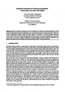
Small values for Metric 1 show a good suitability of the method for the evaluation of quantitative performance requirements. In the following we present the predicted response times for each approach. The times are sorted according to design alternatives and participants, and are shown in a table using bar charts. In the second last column the actual measurements of the web server can be found, which enables the comparison with the predictions. The last column contains the mean deviation of the forecasts from the measurements in percent for each alternative determined among all participants. The bar chart of the last column was generated automatically and does not mean the absolute response times. In figure 1 the response times forecasted with the SPE-approach are presented. With
3,5
End-to-end user time
3,0 2,5 2,0 1,5 1,0 0,5 0,0
1
2
3
4
5
6
7
8
Measurement
Deviation
0: No Optimization
1,1928
2,9415
0,9562
1,3168
1,5503
1,8476
2,3094
0,6845
1,5100
0,3724
1a: Static Cache
1,1883
2,9338
0,9499
1,3108
1,5196
1,8204
2,3030
0,6200
1,5300
0,3700
1b: Dynamic Cache
1,1317
2,8670
0,8981
1,2545
1,4868
1,7826
2,1478
0,5800
1,4400
0,3837
0,9546
1,3482
1,5477
1,8428
2,3944
1,5600
0,2496
2: Single-threaded 3: Compression
0,8188
1,6856
0,7096
0,8766
1,2979
1,1221
1,8822
0,6089
0,8100
0,4822
4: Clustering
1,1952
2,9367
0,9588
1,3152
1,5323
1,8421
1,9892
0,6878
1,6500
0,3317
Participant
Fig. 1. Predicted end-to-end user times, SPE method
this approach several participants did not succeed in computing a response time for design alternative 2 (single-threaded version of the server) since the SPE-approach does not support modelling multiple threads. The deviations in the forecasts of individual participants are based on the fact that the SPE method needs input values, which are not present during the design phase of the system development. These values must be gathered from comparable systems or prototypes or have to be estimated on the basis of
developers’ experiences. In this experiment the input values were estimated by the participants. This explains the large deviations of the predicted values from the measurements. Nevertheless, significant patterns concerning the performance behaviour of the single design alternatives are observable. The Metric 1 computed for the SPE approach amounts to 0,3649. That is, the forecasts deviate on the average over all participants and design alternatives by 36% from the measurements. For the CP-approach the results of only 6 participants were gathered (figure 2) as two of the students were not able to finish their predictions within the available time. Just as with the SPE method, most participants did not succeed in modelling alternative
End-to-end user time
2,0 1,5 1,0 0,5 0,0 1
2
3
4
5
6
Measurement
Deviation
0: No Optimization
1,50536
1,50536
1,50533
1,50524
1,50510
1,50522
1,5100
0,0031
1a: Static Cache
1,50536
1,50536
1,50533
1,50524
1,50510
1,50522
1,5300
0,0162
1b: Dynamic Cache
1,40399
1,40399
1,40397
1,40387
1,40373
1,40386
1,4400
0,0251
1,49110
1,49190
1,5600
0,0439
2: Single-threaded 3: Compression
1,21125
1,26893
1,18273
1,40061
1,98167
1,10916
0,8100
0,6778
4: Clustering
1,45336
1,45336
1,44094
1,44089
1,44082
1,44089
1,6500
0,1242
Participant
Fig. 2. Predicted end-to-end user times, CP method
2 and provided no results. With the CP-approach the forecasts of the participants, except alternative 3, differ very slightly from the measurement of the implementations. That is because of the fact that the method uses data measured on an available system. With alternative 3 a compression rate for delivered files had to be estimated, therefore noticeable deviations in the values arise. Metric 1 computed for the CP-approach amounts to 0,1484. By about 15% deviation of prediction from measurements the CP method suites well for predicting future performance for existing systems. Response times predicted with the umlPSI-approach are presented in figure 3. Apart from the infeasibility of modelling threads, the relatively large variation of obtained results is remarkable. With this approach, input data based on estimation is not separated into software and hardware resources, as it is the case with the SPE approach. In addition, the umlPSI approach relies on less input data, which makes the forecasts more inaccurate. The mean deviation between the predicted and measured response times computed via Metric 1 is here over 500%. To answer question 1 it can be stated that the CP approach is suitable for validation of performance requirements because of its comparatively high accuracy with the
End-to-end user time
25,0
0,5 Req./sec 0,5 Reqf./sec 0,2 Req./sec
0,17 Req./sec
0,06 Req./sec
0,2 Req./sec
0,2 Req./sec
0,17 Req./sec
~1 Req./sec
20,0
15,0
10,0
5,0
0,0 1
2
3
4
5
6
7
8
Measurement
Deviation
0: No Optimization
2,3932
5,4211
10,5690
12,2504
21,1166
6,3678
16,0072
8,7612
1,5100
5,8615
1a: Static Cache
2,3922
5,6192
10,5812
11,6949
21,4039
5,9798
14,3145
8,6219
1,5300
5,5856
1b: Dynamic Cache
2,1750
5,2493
9,7972
10,4271
20,7919
5,9458
13,3239
7,1867
1,4400
5,5015
2: Single-threaded
3,2306
1,5600
1,9865
3: Compression
1,4886
3,1577
8,3245
5,2539
22,2858
5,7347
7,4177
9,3413
0,8100
8,7229
4: Clustering
2,3103
5,0517
9,4992
10,4794
15,3719
5,1540
16,0813
8,2451
1,6500
4,4692
6,0873
Participant
Fig. 3. Predicted end-to-end user times, umlPSI method
forecast of the absolute response times. However, the CP method requires measured response times of an existing system, therefore it can be only used for new developments in later phases of the software development. 4.2
Do the methods really support the decision for the design alternative with the fastest implementation?
On the basis of the predicted response times the design alternatives can be ordered. The question is, how authentic this order is, if compared with performance of the implementation of alternatives. We need a metric indicating the number of wrong decisions suggested by a certain method. For this reason first a ranking for the design alternatives is set up on the basis of the measured response times. Let A be the set of all design alternatives under consideration. We define a mapping P osmeas : A −→ {1, ..., |A|} with P os(AlternativeA) ≤ P os(AlternativeB) for the response time of the alternative B being not less than the one of the alternative A. In the same manner the design alternatives are arranged for each participant into a ranking according to their predicted response times. The mapping P ospredi arranges similarly to each alternative its place in the ranking according to the response times predicted by participant i. In the next step we want to calculate, how many positions the measurement-based ranking differs from the prediction-based ranking. Since we do not want to take into account place permutations in cases of insignificant differences in response times we divide the alternatives according their measured times into classes applying a distancebased clustering algorithm [1]. In this way alternatives with very close response times are regarded equivalent and belong to the same class. The monotonically increasing
mapping Class : P osmeas (A) −→ {∞, ..., |Cla∫ ∫ e∫ |} assigns each position of the measurement-based ranking to the class of the associated design alternative. Subsequently we define Displacementi (Alt) := |Class(P ospredi (Alt)) − Class(P osmeas (Alt))|. This formula indicates for the participant i the number of place discrepancies between his predicted ranking of design alternative Alt and the measurement-based ranking of this alternative if the rank positions belong to different clusters. Metric 2 is defined as follows: n
m2 :=
|A|
1 XX Displacementi (Altj ), n i=1 j=1
Ranking Design Alternatives: 1. (fastest) 2. 3. 4. 5. (slowest) Metric 2:
Class 1 Class 2 Class 2 Class 2 Class 2
Participant 8
Participant 7
Participant 6
Participant 5
Participant 4
Participant 3
Participant 2
Participant 1
Participant 6
Participant 5
Participant 4
Participant 3
umlPSI Participant 2
Participant 1
Participant 8
Participant 7
Participant 6
Participant 5
Participant 4
CP Participant 3
Participant 2
Measurement 3 1b 1a 2 4
SPE Participant 1
Classes
with n being the number of participants predicting with a certain method. The smaller the value of the metric m2 the less false placements were obtained by ordering the alternatives according to timing behaviour. Figure 4 shows the comparison of the measured and the predicted rank lists of our experiment. On the basis of measurements the alternative 3 was assigned to the class 1
3 3 3 3 3 3 3 1b 3 3 3 3 1b 3 3 3 3 3 4 4 3 4 1b 1b 1b 1b 1b 1b 4 3 1b 1b 1b 1b 4 1b 1b 4 4 1b 1b 3 1b 1b 1a 1a 1a 1a 1a 1a 1b 1a 4 4 4 4 2 4 4 1b 1b 4 1a 1b 1a 1a 4 4 2 4 4 4 1a 4 1a 1a 1a 1a 1a 1a 1a 1a 1a 1a 3 1a 4 3 2 2 4 2 2 2 2 2 2 2 2 2 3 2 2 2 2 2 2 2 2 2 0,25 0,33 0,75
Fig. 4. Ranking of design alternatives
and other alternatives to the class 2, because the response time of alternative 3 clearly differs from others. With the SPE and CP approaches there are only two ”‘incorrect”’ placements in the prediction-based ranking of one participant in each case. Other place permutations among the alternatives 1a, 1b, 2 and 4 occur within a cluster and therefore do not taken into account. With the umlPSI approach more often an alternative of the ”‘slower”’ class was forecasted being the fastest, which results in the notably higher value for Metric 2. As answer to question 2 it can be stated that both the SPE and CP approach are well suited for supporting the selection of the best design alternative concerning timing behaviour.
4.3
How does the application of the methods compare to an unmethodical approach to performance prediction?
The tasks of the experiment were additionally given to seven members of the control group, who did not take part in the tutorials. Doing so we wanted to find out whether the intuitive evaluation of design alternatives leads to different decisions than applying one of the methods. The members of the control group did no ranking of the alternatives but selected the best one on their own opinion. Four of the seven members of the control group preferred the alternative 1b (dynamic cache), only three participants picked alternative 3 (compression). Thus, the larger part of the control group took an alternative, which had the best response times in only 12% of the method-supported predictions. Although the sample of seven participants is very small, this result at least implies that analysing the design documents does not lead necessarily to the decision for design alternative 3 and that our experiment’s setup was valid. 4.4
What are the properties of the methods and where is room for improvement?
We grouped the properties of the methods into four different subsections: expressiveness, tool support, domain compatibility and process integration, and report our experiences with them during the experiment. Expressiveness The SPE method has a quite intuitive separation of a software and a system model, which allows changing hardware and software independently for a quick analysis of different designs. The underlying queueing networks are encapsulated by the method’s tool and are not of the developers’ concern. One scenario may be modelled over multiple levels of control flow making it easy to model complex situations. Multiple scenarios on one resource may be evaluated via simulation directly within the tool. Although it is possible to model quite complex systems, the students were not able to model multiple threads within one process. An advanced system model for different queueing disciplines and the inclusion of passive resources has been proposed [15], yet is not implemented in the tool. The SPE method allowed the students to make predictions on the performance of the architecture with the fewest input data of all three analysed methods. Thus it is suitable for application during early development cycles when details of the complete architecture are still unknown. Other than the SPE method, in CP only a system model is used for the analysis. No explicit software model is included. The workload of a system is characterised by traces of requests and the output of monitoring tools. It is necessary to have at least a prototype of the new architecture to collect this data. In our experiment we had to include a workload-trace of a prototype of the web server into the design documents, so that the students could apply the method. Many different queueing networks may be modelled, for example with multiple queues before one server or the blocking of resources. This allows a lot of real-life situations to be analysed. Yet software tools are missing for some of these networks and the analysis has to be done manually in this case. Like in SPE the students had difficulties modelling multiple threads. A hierarchical structuring of complex queueing networks is not provided. Because this method relies on measured
performance data, it is better suited for performance planning when extending existing systems. The expressiveness of the umlPSI approach is as powerful as UML diagrams (usecase-, activity- and deployment-diagrams) and the UML profile used. Using UML was intuitive for the students, who had learned this modelling language in a course about software engineering. Some students complained that the modelling of hardware resources with deployment diagrams was not expressive enough because the UML Performance Profile only allows the definition of a speed-factor to differentiate resources. Multiple threads could be modelled through a passive resource with a pool of threads. The generated simulation is more powerful than the analysis models of the previous two methods. For example, it allows arbitrary distributions of incoming requests, while queueing networks are bound to an exponential distribution. Tool support The SPE-method comes with the tool SPE-ED (Software Performance Engineering EDitor) for Windows, which can be downloaded in a demo version from the authors’ website [13]. The full version for commercial use has to be purchased, yet a price is not provided. SPE-ED has been developed several years ago and the user interface is not up to the latest standards. For example, there is no drag and drop and students complained that the graphical modelling is unintuitive and quite different from similar tools. There is no integration with other modelling tools, although an export function to a XML-based file format has been proposed, but is not implemented yet [16]. Having manually entered software execution graphs the performance modeller is able to do a quick analysis with the tool highlighting expected bottlenecks of his architecture. The tool is stable and the students hardly reported any crashes. A problem of the tool is that it is not possible to feed the performance results directly back into the software model (e.g. in UML) and that software model and performance model have to be maintained separately. Overall, the tool appears useful for serious performance modelling and is the most matured of the analysed tools. Although several tools exist to solve queueing networks, we decided for the CPmethod to use the spreadsheets provided by the authors, which can be downloaded free of charge from their website [9]. There are several versions of the spreadsheets, each one for a different type of queueing network. Spreadsheets are also available for workload clustering as described in the book. The spreadsheets for queueing networks let the user put in the type and number of resources, the expected calculation time on each resource and the arrival rate of incoming requests. They output response times, resource utilizations, queue length and throughput, but do not visualise the results. A graphical visualisation would have been useful because the output may consist of a large amount of numbers, which have to be carefully analysed. Some students reported that they had trouble interpreting the results. Because the queueing networks do not contain an explicit software model and are resource-oriented, reporting back the results into the software model is impossible. The spreadsheets are appropriate for their actual purpose, which is capacity planning for existing information systems. However their usefulness is limited when analysing large software architectures. As mentioned earlier, an UML modelling tool is necessary before using the free umlPSI Linux-tool, because umlPSI only generates and executes simulations out of
XMI-files. Like the authors we used Poseidon for modelling and annotating UMLdiagrams in our experiment. umlPSI in its current implementation is bound to a specific version of Poseidon, since it can only process the XMI-dialect generated by this version properly. The installation of this tool was difficult because it requires some libraries which are not available on every Linux distribution. Most of the students did not manage to install and run umlPSI and only submitted their annotated UML-models exported from Poseidon. Generation and execution of the simulation was also difficult because the tool produced incomprehensible error messages if the XMI-files contained syntax errors, which occurred several times during our testing. After the simulation is executed properly the tool outputs a result table and also reported the results back into the XMI-files, which could be reimported to Poseidon. There the students were able to inspect bottlenecks and make adjustments to their architectures. It would be practical if the tool was available as a plugin for a modelling tool and had not to be started externally. Overall umlPSI is intended as a proof-of-concept implementation for the method and cannot been seen as a tool ready for industrial use. Domain applicability The application domain of the authors of the SPE-method are distributed systems and especially web applications. Their documentation contains several examples of systems providing services to the web. They also documented the application of the SPE-method to embedded real-time systems. The SPE approach is very flexible and can be applied to lots of different contexts. Like SPE, CP is also developed with the focus of web applications and client/server systems as analysis subjects. The authors have written five different books about the topic with varying emphasises (e.g. Web Server, E-Business, Client/Server). The umlPSI tool so far is able to analyse use-case-, activity-, and deploymentdiagrams and is therefore bound to the modelling possibilities of these three diagram types. For example the inclusion of component-diagrams is not possible. The authors tested this method with examples of small web applications. Process integration For the SPE method a well-documented process consisting of several steps is available. Although it is originally designed for the application during the design phase of a waterfall model during software development, the authors also show, that the method can be easily embedded into iterative models like the spiral model or the unified process. CP contains a process model, but it has to be adopted individually depending on the system under analysis. It is best suited to be applied during implementation, testing or evolution stages of a software system. The umlPSI tool can be used every time the developers are concerned with UML modelling, mostly during early stages of the development. It is not bound to a specific process model.
5
Validity of the Experiment
Several limitations affect the validity of our results. We discuss the internal and external validity of our experiment.
The internal validity is the degree, to which every relevant interfering variable could be controlled. This includes the degree to which the results of the experiment are indeed attributed to the properties of the performance prediction methods and not bound to mistakes in our experimental set-up. One interfering variable we could not control was the input to the methods. For the SPE-approach and the umlPSI-approach the students had to base their predictions on estimated values. Instead, for the CP-approach we included a workload trace with measured values into the experimental task, because this is common when applying this approach. The disposition of the students into each group was based on the results of their exercise papers. This way we controlled the possibility of inhomogeneous groups with deviating qualifications. The external validity is the degree, to which the results of the experiment are valid in other situations than the one analysed here. This especially concerns the participants and the analysed subject. The participants in our experiment were students and we could not include practitioners with more experience. However, due to the training session, every student had a similar knowledge about the performance prediction methods. This way, past experiences of the participants did not distort the results, which would have been possible if practitioners had been included into the experiment. The number of students was limited to eight for each method, so a statistical hypothesis test was not possible due to the limited available data points. However, individual exceptions in student performance could be detected in principle. By this the influence of individual performance was controllable. The students analysed a small architecture, the scalability of the methods to larger architectures is unknown. Our implementation of the web server is only one possible implementation, the performance measurements of other implementations of the same design might differ. We analysed only three methods, although more than 20 approaches are known [3]. The validity of our experimental set-up applied to other methods is unknown.
6
Conclusions
In this paper we compared three different methods for the early performance analysis of software systems. A group of students applied the methods on design documents and made performance predictions for the architecture of a web server. After implementing the web server we were able to compare predictions with actual measurements. The SPE method was appropriate to support design decisions. Yet the validation of performance goals was hardly possible because the predictions relied on students’ estimations and a satisfying precision could not be achieved. The method is especially suited for early, explorative predictions because it is able to compute results with only few inputs. A better integration of this method into common modelling tools would be of practical interest.
CP delivered the most precise predictions, but relied on a workload trace of the web server taken from a prototype. Thus, the method is well suited for extending existing system and also able to validate performance goals. But the use for early performance predictions of new architectures is limited. umlPSI might be most convenient for developers because it relies on UML models and does an automatic transformation of software models to performance simulations. However the simulation was more time-consuming than the analysis of the other methods and the tool proved to be error-prone. The umlPSI method can be used during early development cycles, yet the precision of the performance results was the worst in our experiment. Future work in this area includes the conduction of a field study in an industrial environment possibly with a large software architecture. Other methods, especially those for component based systems [5], will also be evaluated. Acknowledgements: We would like to thank Yvette Teiken for implementing the web server, members of the Palladio research group for fruitful discussions and all students, who volunteered to participate in our experiment.
References 1. M.R. Anderberg. Cluster Analysis for Applications. Academic Press, 1973. 2. S. Balsamo, A. DiMarco, P. Inverardi, and M. Simeoni. Model-based performance prediction in software development: A survey. IEEE Transactions on Software Engineering, 30(5):295– 310, May 2004. 3. S. Balsamo, M. Marzolla, A. DiMarco, and P. Inverardi. Experimenting different software architectures performance techniques: A case study. In Proceedings of the Fourth International Workshop on Software and Performance, pages 115–119. ACM Press, 2004. 4. V. R. Basili, G. Caldiera, and H. D. Rombach. The goal question metric approach. Encyclopedia of Software Engineering - 2 Volume Set, pages 528–532, 1994. 5. A. Bertolino and R. Mirandola. Cb-spe tool: Putting component-based performance engineering into practice. In Ivica Crnkovic, Judith A. Stafford, Heinz W. Schmidt, and Kurt C. Wallnau, editors, Component-Based Software Engineering, 7th International Symposium, CBSE 2004, Edinburgh, UK, May 24-25, 2004, Proceedings, volume 3054 of Lecture Notes in Computer Science, pages 233–248. Springer, 2004. 6. I. Gorton and A. Liu. Performance evaluation of alternative component architectures for enterprise javabean applications. IEEE Internet Computing, 7(3):18–23, 2003. 7. H. Koziolek. Empirische bewertung von performance-analyseverfahren f¨ur softwarearchitekturen. Diploma thesis, University of Oldenburg, Faculty II, Department of Computing Science, Okt. 2004. 8. M. Marzolla. Simulation-Based Performance Modeling of UML Software Architectures. PhD thesis, Universit‘a Ca Foscari di Venezia, 2004. 9. D. A. Menasc´e, V. A. F. Almeida, and L. W. Dowdy. Download files for the book: Performance by design: computer capacity planning by example. http://cs.gmu.edu/ menasce/perfbyd/efiles.html, 2004. 10. D. A. Menasce, V. A. F. Almeida, and L. W. Dowdy. Performance by Design. Prentice Hall, 2004. 11. D. A. Menasce and V. A.F. Almeida. Capacity Planning for Web Services. Prentice-Hall, 2002.
12. Object Management Group OMG. Uml profile for schedulability, performance and time. http://www.omg.org/cgi-bin/doc?formal/2003-09-01, 2003. 13. C. U. Smith. Spe·ed: The software performance engineering (spe) tool. http://www.perfeng.com/sped.htm, Jan 2000. 14. C. U. Smith. Performance Solutions: A Practical Guide To Creating Responsive, Scalable Software. Addison-Wesley, 2002. 15. C. U. Smith. Spe-ed user guide. http://www.perfeng.com/papers/manual.zip, 2003. 16. C. U. Smith and C. M. Llad´o. Performance model interchange format (pmif 2.0): Xml definition and implementation. Technical report, Performance Engineering Services, Universitat Illes Balears, 2004. 17. C. Wohling, P. Runeson, M. H¨ost, M.C. Ohlsson, B. Regnell, and A. Wesslen. Experimentation in Software Engineering – An Introduction. Kluwer Academic Publishers, 2000.