Empirical Parameterization of Multi-Agent Models in Applied Development Research
Thomas Berger University of Hohenheim, Germany (
[email protected])
Pepijn Schreinemachers Center for Development Research, University of Bonn, Germany (
[email protected])
Paper for the workshop “Empirical techniques for testing agent based models” Bloomington campus of Indiana University, June 2-4, 2005
Empirical Parameterization of Multi-Agent Models in Applied Development Research Abstract An important goal of modeling human-environment interactions is to provide scientific information to policymakers and stakeholders in order to better support their planning and decision-making processes. Modern technologies in the fields of GIS and data processing, together with an increasing amount of accessible information, have the potential to meet the varying information needs of policymakers and stakeholders. Multi-agent modeling holds the promise of providing an enhanced collaborative framework in which planners, modelers, and stakeholders may learn and interact. The models’ agent behavior is not hidden in differential equations, but can be directly observed. Human actors should therefore be able to identify with their analogs in the computer model. The fulfillment of this promise depends on the empirical parameterization of multi-agent models. Although multi-agent models have been widely applied in experimental and hypothetical settings, only few studies have tried to build empirically based multi-agent models and the literature on methods of empirical parameterization is therefore limited. This paper presents a novel approach for the parameterization of empirical multi-agent models. We employ a Common Sampling Frame to randomly select observation units for both
biophysical
measurement
and
socioeconomic
surveys.
The
biophysical
measurements (here: soil properties) are then extrapolated over the landscape using multiple regressions and a Digital Elevation Model. The socioeconomic surveys are used to estimate probability functions for key characteristics of human actors, which are then assigned to the model agents with Monte-Carlo techniques. This approach generates a landscape and agent populations that are statistically consistent with empirical observation. Validations tests are finally used to assess the sensitivity of model results to possible measurement error.
2
1. Introduction In applied development research we often find critical triangle situations of poverty, resource depletion and decreasing productivity (Vosti et al., 1997). Poor farm households are compelled to apply unsustainable farming practices, which erode their natural resource base, reduce crop yields, and in turn, promote poverty. In many developing countries, especially in Sub-Saharan Africa, farm households are trapped in such a downward spiral of interacting biophysical and socioeconomic forces (Pender et al., 2004). A major research issue in agricultural and development economics is to explore policy options to overcome this critical triangle and, in particular, to analyze the likely impacts of innovations on the livelihood of farm households and their natural resource conditions. Whereas in the past, research mainly focused on technical innovations, more emphasis is currently paid to institutional innovations, such as land rental and labor sharing arrangements, resource user associations and catchment management boards. Multi-agent system models—in the following abbreviated with MAS—have a large potential to improve the understanding of complex agro-ecological systems, to learn about the uncertainties related with natural resource management and to explore new policy options (Parker et al, 2003). They may also provide a collaborative learning framework in which scientists, policy makers and stakeholders may interact (Roeling, 1999; Hazell et al., 2001; van Paassen, 2004). To fulfill their potential, multi-agent systems need to be carefully parameterized and validated with empirical data. Only then they may provide relevant information about boundary conditions of rural development and the uncertainties involved. MAS have been widely applied in hypothetical and experimental settings; only few studies have tried to build empirically based multi-agent models, and the literature on methods of empirical parameterization is therefore limited (Berger and Parker, 2002). We argue in this paper that MAS can, and should, build on the large body of literature on applied development research, such as social network studies, rural sociology, agricultural economics, agronomy, crop, soil and animal sciences and farm engineering. There is no need to reinvent the wheel. The need is to integrate well-established, sound 3
methods of applied development research within a multi-agent framework. The added value from integrating empirical research methods is yet scarcely exploited, and multiagent systems clearly have a potential for doing this. Even more so, the use of wellestablished disciplinary methods and integrating them within a multi-agent framework increases the acceptance of multi-agent research by scholars not yet convinced of this approach. The paper is organized as follows. Section 2 introduces whole-farm mathematical programming as an appropriate method for incorporating bio-physical and socioeconomic data and processes based on empirical measurements and observations. Section 3 discusses the peculiarities of developing country research and proposes the use of Common Sampling Frames as a suitable method for organizing data collection in interdisciplinary research projects. We then present a novel approach – based on spatial interpolation and Monte-Carlo techniques – to parameterize MAS with empirical data. Taking the example of ongoing research in Uganda, we show how landscapes and agent populations can be generated from field measurements and farm household survey data. The last section discusses the validation of our approach and concludes.
2. Integrated Modeling and Empirical Multi-Agent Models The application of computer models has a long tradition in agricultural sciences and high standards for model parameterization and validation have been established. Computer models in agricultural sciences have always been tailored to provide ‘practical’ results for applied development problems. Crop growth models, for example, are used to simulate the fertilizer response of major food crops – thereby substituting for costly field experiments – and Linear Programming models are used to derive improved farm management plans. There is also vast experience with the coupling of these computer models, for example in bio-economic models (Barbier, 1998; Woelcke, 2003; Holden and Shiferaw, 2004) and in integrated river basin models (Rosegrant 2000; Fischer et al., 2002).
4
Integrated modeling of natural resource use In general, integrated models in agricultural sciences have been very instrumental in capturing the technical or engineering aspects of human-nature interactions and in highlighting the economic consequences of resource use changes (Kuyvenhoven et al., 1998). They may elucidate the tradeoffs that farm households face in crop choice and farming practices, assess the profitability of various land-use options and capture the internal costs of adjusting to changes in environmental and marketing conditions (see also the more recent work of Holden et al., 2004; Deybe and Barbier, 2005). But they face also limitations when it comes to analyzing critical triangle situations, in which heterogeneity of actors and landscapes is large and increasing (Berger et al., 2005). In general, this is the case when farm households differ considerably in terms of factor endowments and decision-making processes and when resources are exchanged locally or in networks. Another challenge for integrated modeling is to allow for a sufficient degree of spatial and temporal complexity, since changes in the natural environment, the market environment, and the introduction of improved technologies typically involve long-term interacting processes.
Heterogeneity and interactions clearly fall into the core competence of multi-agent models, which may therefore extend the scope of computer modeling in applied development research. In the field of natural resource use, multi-agent models have been applied to a variety of research questions (for an overview see Janssen, 2002; Parker et al., 2003). Multi-agent models have been applied to theorize about social and spatial dynamics (Gotts et al., 2003; Parker and Meretsky, 2004), to simulate land-use changes (Huigen, 2004), to assess the impact of agricultural policies (Balmann 1997; Berger, 2001; Happe et al., 2004), to accompany role-playing games (Barreteau et al., 2003) and in game theory applications (Bousquet et al., 2001). According to the classification proposed by Berger and Parker (2002), most of these applications are abstract or experimental; only few studies have tried to build empirical multi-agent systems. Moreover, there are only few studies that have attempted to exploit the potential of multiagent systems in integrating biophysical and socioeconomic model components (Parker and Berger, 2002) 5
In the remainder of this section we will first introduce Mathematical Programming as an appropriate format for integrating biophysical and socioeconomic data and processes and then list the particular challenges to building empirical MAS Mathematical programming A mathematical programming model maximizes an objective function subject to constraints. A mathematical program of a farm household usually maximizes gross margins, household income or utility. Variables in the objective function include alternative economic decisions, such as production and consumption decisions, which are called activities. Activities typically include the growing of crops under different input levels, selling of farm produce and purchasing of consumption goods, renting in and renting out land or labor, etc. Solving the mathematical program implies the selection of a range of activities that yields the highest value of the objective function. The selection of activities is constrained by a number of equations. For instance, no more area can be planted to crops than is available in land and no more products can be sold than what is produced. These constraints also include many technical details such as fertilizer application rates per crop, the level of crop yield for specific input combinations, nutrient extraction per unit of land. A mathematical program of the farm household can thereby simulate farm household decision-making in all its biophysical and socioeconomic aspects, such as land use, off-farm labor, investment and consumption. For an excellent introduction to mathematical programming of the farm household, the reader is referred to Hazell and Norton (1986).
The main advantage of using the mathematical programming format is that it builds on a common way of thinking about agricultural activities and natural resource use. Farmers, agronomists, and extension workers on the one hand, crop scientists and agricultural economists on the other, are familiar with posing their problems and research questions in this format. Whole-farm mathematical programming is a well-established “natural” framework for organizing quantitative information about the production and consumption side of agriculture. It may therefore serve as the basis for integrating different types of 6
knowledge into a common framework and to represent real-world farm households in multi-agent systems. We will come back to the prospects of model-enhanced learning in the concluding section of this paper.
Challenges to building empirical MAS When building empirical MAS four special challenges arise: 1. Empirical parameterization: the cellular and the agent-based component of the MAS need to represent a real-world situation of typically heterogeneous biophysical and socioeconomic conditions, for example, various soil types, crop and vegetation growth, land holdings, social networks and human actors. 2. Simulating real-word decision problems: agent decision-making needs to capture the essential features of real-world complexity and trade-offs such as – in the case of rural development – investment versus consumption, subsistence versus market production, short-term profit versus ecological sustainability. 3. Model validation: the MAS needs to be validated against empirical data. Simulation result should resemble real-world development paths and show a sufficient goodness of fit in baseline scenario. 4. Sensitivity testing: empirical data have measurement errors and not all model parameters are known. Simulation results therefore need to be checked for these uncertainties. This paper elaborates in detail on the first two challenges and outlines how the remaining challenges might be approached.
3. Collection of empirical data As mentioned in the previous section, MAS has a large potential for integrated modeling of land-use changes based on empirical data. Although the capabilities of present-day technology, such as GIS and related data processing tools, have made more biophysical information than before accessible, there are still some challenges for data collection especially in interdisciplinary research projects. 7
Common Sampling Frame One drawback of doing applied research in developing countries is data scarcity. Statistical agencies in developing countries are limited in resources and often rely on donors to conduct surveys. Data quality is generally poor as farm households do not keep records and the informal sector forms a large part of the economy. Time series data are mostly for short periods because funding has been variable and political instability has frequently interrupted continuous data collection. Data collection—for example, through living standard measurement surveys—has much improved recently, yet large data gaps remain. Under the condition of data scarcity, scientists in interdisciplinary research projects do best to concentrate their primary data collection on selected sites. But one tendency is that scientist from various disciplines use different criteria for selecting their units of observation. As a result, data collection activities are often scattered over the study region, soil samples are taken from different villages than those villages surveyed by the social scientists, plant growth models are calibrated for selected crops not grown by trial farmers etc. Under these conditions—which are unfortunately rather the rule than the exception—it becomes very difficult to create consistently integrated datasets and to empirically parameterize multi-agent models. One way out is to apply a statistical procedure to select representative units and subunits of observation using a common sampling frame. This approach was employed for data collection in the Ghanaian Volta basin in West Africa as described in Berger et al. (2002) and Vlek et al. (2004). First, a priori information was compiled and merged—here: living standard measurements and publicly available geospatial information. Project scientists then developed a hierarchy of observation units (Figure 1) and defined selection criteria that from a theoretical point of view would potentially capture all key research aspects of the various scientific disciplines involved. Based on preliminary analysis of the merged data set, a set of operational selection criteria at the community level was identified belonging to the following categories: agro-ecological conditions, agricultural and fishing 8
intensity, market orientation, household welfare, health and water use, social capital, and migration. Initial correlation analysis of the merged data set revealed interdependences among some of the selection criteria, and Principal Component Analysis was therefore used to derive a relatively small number of linear combinations of the original variables that retain as much statistical information as possible. Eight new variables, explaining about 70% of the total variance in the data, were used for a subsequent Cluster Analysis. The communities closest to the cluster centroid were then selected as representative communities proportional to the size of their cluster. Scientists of the various disciplinary sub-projects then randomly selected their sub-observation units within these sample communities, for example households, water sources or sample plots.
Scale 1,000 km
100 km
10 km
1 km
0 km
Social systems
Ecological systems
Country | Region | District | Community | Village | Household | Technology Livestock Plot
River Basin | Sub-basin | Landscape | Sub-catchment | Hydrology Response Unit | Farming systems | Plot | Point sample (subplot) Observation units
Figure 1: Hierarchy of observation units in interdisciplinary research
The advantage of this interdisciplinary approach, apart from the logistical benefits that accrue from the concentration of field activities at community level, is that it provides representative and integrated data sets for the empirical parameterization of MAS. In the following subsection we briefly explain how we combined soil samples and farm household surveys at the community level. The sampling framework for this case study in Uganda was constructed slightly different than in Ghana, and the sites selected for MAS 9
research were added to the sample because they were part of longer-term farm trials of the International Center for Tropical Agriculture (Ruecker, 2005). But the approach is fundamentally the same; a GIS-based statistical stratification was used to select representative communities in which natural and social scientists would then collect their primary data from the same observation units.
A case study from Southeastern Uganda The remainder of this paper describes a novel methodology that combines predictive soil maps to generate a landscape from soil samples, and Monte Carlo techniques to generate agent populations from a sample of farm households. The method is described on the basis of a case study on two village communities in the Lake Victoria Crescent of Southeastern Uganda. The two village communities are Magada and Buyemba; both are located in the southern part of the Iganga District, which through redistricting has recently become the Mayuge District. The two communities are relatively well connected to Mayuge and Iganga town, which gives farm household relatively good access to markets. The first farm families settled in Magada in the early 1920s. Settlers mostly followed the paths created by seasonally migrating buffalo. The first families settled at some distance from these paths for enhanced safety, with later arrivals settling more land inward or directly along the path. Buyemba was populated later, in the 1950s. Magada counts around 374 households, which is somewhat more than the 247 households residing in the smaller village of Buyemba. Both communities are densely populated with an average 436 and 383 people/km2 in Magada and Buyemba, respectively. Climatic conditions allow the cultivation of two sequential crops in a year. Main food crops are cassava, sweet potato and beans, the main cash crops is coffee, while maize and plantain are both sold and home consumed. Farm households predominantly rely on the hand hoe in their crop management, the use of external inputs such as fertilizers, pesticides and improved seeds is rare. Intercropping is common and farm households usually allocate only small parts of a plot to a single crop combination. The dominant soil 10
texture is sandy clay loam (Ruecker 2005). The soil fertility is generally low but varies across locations in the community. The landscape is moderately sloping with large flat areas. Erosion levels are moderate (Brunner 2004, Ruecker 2005). 4. Generation of landscapes in MAS In the MAS a landscape of grid cells represents the biophysical environment that farm households manage. The landscape is organized in spatial layers with each layer containing the information about a specific property. In the Uganda study, the landscape comprises two village communities which together occupy about 12 square kilometers. The landscape model contains 12 layers, including soil chemical and physical properties, village boundaries and the location of farmsteads and agricultural plots. Layers are composed of grid cells. By defining the grid cells sufficiently small, the raster format is as good as the polygon format. The grid cell size in the Uganda study is, for example, set to 71 x 71 meters (0.5 ha), which is the smallest amount of land cultivated by a single farm household. From soil samples to continuous soil maps Empirical information about soil properties is obtained from soil samples. The challenge here is to create continuous soil maps by interpolating soil sample values. There are various approaches to this, such as a kriging interpolation using semivariogram models or distance weighting algorithms (e.g., Ruecker 2005). The Uganda study used predictive soil mapping based on stepwise multiple regressions of soil properties on terrain parameters and/or other soil properties (Rhew et al. 2004). Terrain parameters were derived from a Digital Elevation Model (DEM) and included elevation, slope, upslope area, plan curvature, profile curvature, curvature, wetness index, streampower index, and aspect. In a first stage, the prediction was based on 285 soil samples and 910 GPS measurements from a single hillslope in the village of Magada collected in 2000 (Ruecker 2005). Predictive models were initially estimated from these data and scaling effects were explored to find robust estimators at different scales. 11
In a second stage, a new round of 120 soil samples and GPS measurements were collected in two villages in 2003. These data were used to validate the predictive models of the first stage, and to subsequently modify these (Rhew et al. 2004). In addition, these data were used to establish pedo-transfer functions for phosphorus (idem.). Distribution of agents into the landscape The second challenge is to populate the landscape with agents. The location of farmsteads and agricultural plots can be obtained through GPS measurement, maps of the land registry office, or aerial photography, yet such information is often unavailable. In the Uganda study, hand drawn maps were available on which most of the sample households had been marked during the survey but not the exact location of their plots. The maps, however, showed that farmsteads were mainly located along community roads with scattered farmsteads in the other parts of the villages. The remaining 83 percent of the farmsteads and all the plots were thus be assigned using these qualitative patterns (in ongoing research in Chile complete geo-referencing of household surveys and land registry maps are used). When complete data sets are lacking, random assignment is an option and subsequent sensitivity testing to repeated random assignments can reveal the impact of this unknown factor on eventual simulation outcomes. A complete random assignment is, however, inappropriate because of spatial dependency; farmsteads are clustered around the road network and this has to be taken into account. Figure 2 shows the different stages in generating the spatially located agents and farm plots for the village of Magada; the same procedure was applied to Buyemba. The left upper panel (Figure 2A) shows the sample points within the village boundary of Magada. The figure shows that sample farm households are not evenly distributed in the landscape but are clustered around the road network. The figure only shows main roads, but it should be noted that the cluster of dots in the north and center of the village are also close to smaller roads. 12
Two different areas according to population density are therefore first demarcated: areas alongside the road network are designated as of high population density, and all other areas are of low population density. Assuming that farm households were randomly selected, the geographical distribution of the sample households represents the distribution of the total population. In Magada, for instance, 84 percent of the sample households live in the high-density area, which accounts for 40 percent of the total village area. Of the remaining (non-sample) households, 84 percent is thus allocated in the high-density area and 16 percent in the low-density area (Figure 2B). This methodology created a problem in the village of Magada in that the estimated area from the survey much exceeded the available area within the village boundary, no such problem arose for Buyemba. The likely explanation is that many farmsteads in Magada, unlike in Buyemba, are located close to the village boundary in the north of the village: these farm households might have plots outsides of the village boundary, which are included in our survey data. The data were therefore adjusted by randomly deleting 95 (non-sample) agents from the population so that the total estimated and available areas matched. Figure 2B shows the agent population after this adjustment. All allocated farmsteads were then converted into grid cells, as shown in Figure 2C. Each agent becomes a unique identification code at this stage. Finally, using the estimated sample distribution from the survey, agricultural plots were allocated to the agents. The spatial randomizer was not used at this stage, as this would have produced an unrealistically scattered pattern of farm plots. The allocation was therefore done manually (Figure 2D). Sensitivity analysis is applied to reallocate plots to different agents but not to redraw the map.
13
A. Survey sampling points
B. Random allocation of other points
C. Location of farmsteads
D. Distribution of agricultural plots
Figure 2: Spatial generation of agent population and agricultural plots from a sample of farm households
5. Generation of agent populations in MAS When generating an empirically based MAS, every computational agent must represent a single real-world farm household. Data are not usually available for every farm household but only for a sample of them. In the Uganda study, data were available for only 17 percent of the farm households. The challenge hence is, to extrapolate the sample population to parameterize the remaining 83 percent of the farm households.
14
Watch out for the clones The most obvious strategy would be to multiply every farm households in the sample by a factor six, or if the sample is not random, by the inverse of every observation’s probability weight. Average values in such agent population would exactly equal those of the sample survey. This copy-and-paste procedure is, however, unsatisfactory for the several reasons. First, it reduces the variability in the population. A sampling fraction of 17 percent gives six identical agents, or clones, in the agent population. This might affect the simulated system dynamics, as these agents are likely to behave analogously. It becomes difficult then to interpret, for instance, a structural break in simulation outcomes: is the structural break endogenous, caused by agents breaking with their path dependency, or is the break simply a computational artifact resulting from the fact that many agents are the same? This setback becomes the more serious the smaller the sampling fraction is, because a higher share of the agents is identical. Second, the random sample contains a sampling error of unknown magnitude, which is also multiplied in the procedure. When using the copy-and-paste procedure, only a single agent population can be created, while for sensitivity analyses a multitude of alternative agent populations is needed. For these reasons, the procedure for generating agent populations is automated using Monte Carlo techniques, to generate a whole collection of possible agent populations. Monte Carlo approach Monte Carlo studies are generally used to test the properties of estimates based on small samples. It is thus well suited to this study, where data about a relatively small sample of farm households is available but the interest goes to the properties of an entire population. The first stage in a Monte Carlo study is modeling the data generating process, and the second stage is the creation of artificial sets of data. The methodology is based on empirical cumulative distribution functions. Figure 3 illustrates such a function for the distribution of goats over farm households. The figure 15
shows that 35 percent of the farm households in the sample have no goats; the following 8 percent has one goat, etc. This function can be used to randomly distribute goats over agents, as well as all other resources in an agent population. For this, a random integer between 0 and 100 is drawn for each agent and the number of goats is then read from the y-axis. Repeating this procedure many times recreates the depicted empirical distribution function.
Figure 3: Empirical cumulative distribution of goats over all households in the sample Each resource can be allocated with this procedure. Yet, each resource would than be allocated independently, excluding the event of possible correlations between different resources. However, actual resource endowments typically correlate, for example, larger households have more livestock and more land. To include these correlations in the agent populations, first the resource that most strongly correlate with all other resources are identified and used to divide the survey population into a number of clusters. Empirical cumulative distribution functions are then calculated for each cluster of sample observations. In the Uganda study, the sample is divided into clusters defined by household size because this is the variable most strongly correlated with all other variables. Cluster analysis can also be used for this purpose if several variables show strong correlations, but clusters produced under this procedure are more difficult to interpret, especially when many variables are used. Nine clusters were chosen, as this number captures most of the different household sizes and allocates at least five observations to each cluster. 16
Each agent is allocated quantities of up to 80 different resources in the random procedure. These resources include 68 different categories of household members (34 age groups of two sexes), 4 livestock types (goats, young rams, cows, and young bulls), an area under coffee plantation, female head, liquidity, leverage, and innovativeness. Agents are generated sequentially, that is, agent Nr.1 first draws 80 random numbers in 80 different cumulative distribution functions before agent Nr. 2 does the same. As most resources only come in discrete units, a piecewise linear segmentation is used to implement the distribution functions. Five segments were chosen as this captured most resource levels; more segments would be needed if the number of resource levels per cluster is larger than five or if many resources have continuous functions.
Figure 4: Empirical cumulative distribution functions of goat numbers over nine clusters by household size Consistency checks In order to get realistic agents, four tools are available in addition to the cluster-specific empirical cumulative distribution functions for each resource. First, checks for inconsistencies at the agent-level. An agent with 20 household members is very unlikely to have only one plot of land. Yet, because of the purposeful randomness of the resource allocation, unrealistic settings can occur in the agent population. By defining a lower 17
and/or upper bound for some combinations, this problem can be overcome. If a resource combination lies outside such bound the generated agent is rejected, and the procedure is repeated. Two sets of bounds are included. The first set defines minimum land requirements for livestock and the second set defines demographic rules to ensure realistic family compositions. Second, checks for inconsistencies at the cluster level. The generated mean resource endowments have to lie within the confidence interval of the estimated sample mean; and the correlation matrix of the agent population has to reflect the correlation matrix of the sample population. If not, the generated agent population is rejected. Third, checks for inconsistencies at the population level. The mean resource endowments of the agent population have to lie within the confidence intervals of each estimated sample mean. Fourth, if individual agents, clusters of agents or entire agent populations are continuously being rejected on one of the above criteria, then the cluster-specific distribution functions can be fine-tuned. 6. Results To test the methodology, a large number of agent populations was generated by applying different random seed values. Their properties are analyzed at three levels: 1) the population level; 2) the cluster level; and 3) the level of the individual agents. Each of these is discussed in the following. It was not attempted to show the entire variation between and within agent populations. Instead, the results are illustrated with a few examples and snap shots from the agent populations. Population level At the population level, it is checked whether the averages in the agent population resemble those of the survey population. For this, average resource allocations for hundred generated agent populations were calculated in Table 1. For all resources, the 18
average resource endowments in the agent population fall within the confidence interval of the survey average and the difference between the two averages is generally small. The random agent generator hence reproduces population averages.
Table 1: Resource endowments of the survey population compared to metaaverages of the agent population Resource Household members % children Cows Young bulls Goats Young rams Coffee, ha Plots, 0.5 ha Innovativeness
Population
Average
SE SD1
Survey
7.87
0.45
Agent
7.89
0.11
Survey
55.06
2.47
Agent
54.87
0.75
Survey
0.81
0.18
Agent
0.81
0.02
Survey
0.08
0.04
Agent
0.09
0.01
Survey
1.29
0.16
Agent
1.23
0.04
Survey
0.14
0.04
Agent
0.14
0.02
Survey
0.31
0.10
Agent
0.31
0.02
Survey
4.58
0.51
Agent
4.34
0.00
Survey
3.88
0.17
Agent
3.85
0.04
Confidence interval 6.99
8.75
50.22
59.91
0.45
1.17
0.01
0.16
0.98
1.61
0.06
0.23
0.11
0.51
3.58
5.58
2.35
3.03
Note: Agent population is average over 100 different agent populations. 1
SE is Standard Error of the average referring to the average within the survey population; SD is Standard Deviation of the average
referring to the average across agent populations.
To get more detail about the demographic structure of the population, a population pyramid for the survey population is calculated and compared with one agent population in Figure 5. This form of presentation may not be very suitable for comparing age groups exactly but does illustrate the striking similarity between the two populations.
19
Figure 5: Population pyramids for survey and one agent population compared Cluster level The above has shown that the sample population is well replicated at the aggregate population level, but it is not necessarily so at lower levels of aggregation. The following graphs and figures thus look at the cluster and agent level. Figure 6 depicts four boxplots comparing the distribution of household size, area under coffee, goats and cows in the sample with an agent population with seed value 577. Each box ranges from the 25th to the 75th percentile (the inter-quartile range) with the 50th percentile, or median, also marked in it. Clusters are formed by groups of household size, which is why there is a strong correlation between these two variables in the left upper pane. The figure shows that median values do not differ much between the survey population and the agent population. In addition, most inter-quartile ranges are of comparable width, except for household size, but that is because this variable was used to define the clusters.
20
Note: Graphs show minimum, maximum, interquartile range (bar) and median value (squares)
Figure 6: Boxplots for the distribution of the four major resources over clusters Agent level Agents are patches in the landscape before the non-land resources are allocated. The land endowment is constant for each agent in each subsequent agent population. Non-land resources are allocated to the agent based on the assignment to a household-size-cluster. This assignment is random, with the probability of assignment calculated from the distribution of land sizes over the clusters in the farm survey. Figure 7 plots household size against the number of plots per agent.
21
Note: scatter plots including a linear regression fit
Figure 7: Correlation between household size and amount of arable land One objective for generating agents randomly was to endow each agent differently in different agent populations to allow for sensitivity analysis. Our success in this light is illustrated with Figure 8; this figure is a boxplot showing the variation in resource endowments for agent Nr.250 in hundred generations of different populations. Agent Nr.250 has a fixed location for farmstead and plots as can be seen from the zero variance the agent’s land area of 5 ha. The agent is randomly assigned to alternative clusters, though mostly it is assigned to cluster numbers 0, 1, 2 or 3, because these clusters have most agents with 5 ha of land, that is, these clusters have the highest probability that an agent with 5 ha of land is assigned to them. Because of different cluster assignments and random allocation of resources within each cluster, the variation in resource endowments is high. For example, Agent Nr.250 has a household between 1 and 16 members and between 0 and 5 goats, the level of innovativeness varies from 1 to 5.
22
Figure 8: Boxplot illustrating the variation in agent endowments in alternative agent populations The reproduction of correlations is the third objective in the random agent generation. Figure 9 the left diagram plots the number of adults against the number of children in the survey population, while the two right panes do the same for two generated agent populations with different seed values. The figures show that correlation between adults and children within the household is well replicated in the agent populations, ensuring that
the
agents
created
are
demographically
consistent
in
this
respect.
Note: Scatter plots including a linear regression fit
Figure 9: Scatter plots correlating the number of children and adults, with
23
7. Discussion and Conclusion Multi-agent systems have a large potential for improving the understanding of complex agro-ecological systems. Yet to fulfill their potential, multi-agent systems need to be carefully parameterized with and validated against empirical data. Most multi-agent systems have been based on hypothetical settings using artificial rather than real data. This paper, however, showed that multi-agent systems can also represent real-world conditions by empirically parameterizing agents which represent real-world farm households. The paper outlined a method to generate agent populations from farm household survey data in combination with spatial data on the location of plots and farmsteads and the quality of soils.
When building an empirical multi-agent system in a developing country context, certain challenges arise. As the literature on empirical multi-agent systems is small, these challenges have not been adequately dealt with. Addressing these challenges will be crucial for multi-agent systems to become accepted in the respective disciplinary fields. One such challenge is data scarcity in developing countries. Data are often lacking for calibrating a multi-agent systems and especially for validating the simulation results. As argued in this paper, a common sampling frame is advisable for new research projects, but multi-agent systems are often build on top of existing projects with inherent data gaps.
Even if empirical data are available, validating a multi-agent system remains another challenge. No standard procedures have so far been proposed for validating empirical multi-agent systems. Traditions in validating biophysical components are very different from those for validating socioeconomic components, and standards differ. A related challenge is testing the robustness of the model results to parameter changes. A computer model with many different components has also many parameters, with an inherent level of uncertainty. Model results need to be tested against this uncertainty but the number of tests increases exponentially with the number of parameters. Again, this paper showed how empirical parameterization based on Monte-Carlo techniques may be used for robustness tests. 24
We would like to conclude by briefly commenting on experimental versus empirical MAS. As argued in Parker and Berger (2002), experimental MAS help to integrate “local” knowledge and empirical MAS help to integrate “scientific” knowledge. We do not believe that there is a dichotomy of “soft” and “hard” modeling in applied development research as suggested, for example, by Roeling (1999). MAS could be implemented in such a way that they may be used for both purposes; with computational agents that behave according to heuristics articulated by stakeholders during companion modeling sessions and with computational agents that are empirically parameterized based on survey data and some microeconomic theory as in this paper. Since the model structure is identical, model users and stakeholders should be able to identify with their analogs in both experimental and empirical MAS. This direct interpretability offers exciting prospects for using a combination of experimental and empirical multi-agent methods in collaborative learning processes: to create a platform for exchanging views and perceptions, parameterize the models’ agent behavior and to feed-back scientific findings about inherent system dynamics and resource use externalities.
References Balmann, A. (1997): Farm-based modelling of regional structural change: A cellular automata approach. European Review of Agricultural Economics 24, 85-108. Barbier, B., 1998. Induced Innovation and Land Degradation: Results from a Bioeconomic Model of a Village in West Africa, Agricultural Economics, 19:15-25. Barreteau, O., Le Page, C., D'Aquino, P. (2003): Role-Playing Games, Models and Negotiation Processes. Journal of Artificial Societies and Social Simulation 6(2) Berger, T. (2001): Agent-based spatial models applied to agriculture: a simulation tool for technology diffusion, resource use changes and policy analysis. Agricultural Economics 25 (2/3), 245-260. Berger, T., Parker, D.C., 2002. Examples of Specific Research – Introduction. In: Parker, D.C., Berger, T., Manson, S.M. (Eds.): Agent-Based Models of Land Use / Land Cover
25
Change.
LUCC
Report
Series
No.
6,
Louvain-la-Neuve.
http://www.indiana.edu/%7Eact/focus1/ABM_Report6.pdf Berger, T., Schreinemachers, P., Woelcke, J. (2005): Multi-Agent Simulation for Development of Less-Favored Areas. In: Van Keulen, H. (Ed.): Development Strategies for Less-Favored Areas. Agricultural Systems, Special Issue (accepted for publication). Bousquet, F., Lifran, R., Tidball, M., Thoyer, S., Antona, M. (2001): Agent-based modelling, game theory and natural resource management issues. Journal of Artificial Societies
and
Social
Simulation
vol.
4,
no.
2,
Brunner, A. (2004): Soil erosion in Uganda—From modelling to adapted slope use. ZEF News 16, October 2004: http://www.zef.de/fileadmin/webfiles/downloads/zefnews/no1604-2004-engl.pdf Deybe, D., Barbier.B. 2005. Micro-macro linkages in bio-economic development policy, Agricultural Systems, Special issue on less-favoured areas. In: Van Keulen, H. (Ed.): Development Strategies for Less-Favored Areas. Agricultural Systems, Special Issue (accepted for publication). Fisher, F.M., Arlosoroff, S., Eckstein, Z., Haddadin, M., Hamati, S.G., Huber-Lee, A., Jarrar, A., Jayyousi, A., Shamir, U., Wesseling,H. (2002): Optimal water management and conflict resolution: The Middle East Water Project. Water Resources Research, 38(11): 1243-. Gotts, N.M., Polhill, J.G., Law , A.N.R. (2003): Agent-Based Simulation in the Study of Social Dilemmas. Artificial Intelligence Review 19(1): 3 – 92 Happe, K., Balmann, A., Kellermann, K. (2004): An agent-based analysis of different direct payment schemes for the German region Hohenlohe. In: van Huylenbroeck, G., Verbeke, W., Lauwers, L. (Eds.): Role of Institutions in Rural Policies and Agricultural Markets, Proceedings of the 80th EAAE Seminar "New Policies and Institutions for European Agriculture", Ghent/Belgium, 24.-26.09.2003, Amsterdam/Niederlande: 171182 Hazell, P.B.R., Chakravorty, U., Dixon, J., Celis, R. (2001): Monitoring systems for managing natural resources: economics, indicators and environmental externalities in a 26
Costa Rican watershed. EPTD Discussion Paper 73, International Food Policy Research Institute. Hazell, P.B.R., Norton, R., (1986): Mathematical Programming for Economic Analysis in Agriculture. Macmillan, New York. http://www.ifpri.org/pubs/otherpubs/mathprog.htm Holden, S., Shiferaw, B., 2004. Land degradation, drought and food security in a lessfavored area in the Ethiopian highlands: a bio-economic model with market imperfections. Agricultural Economics, 30(1): 31:49. Holden, S., Shiferaw, B., Pender, J., 2004. Non-farm income, household welfare, and sustainable land management in a less-favored area in the Ethiopian highlands. Food Policy, 19(4), Special Issue: 369-392. Huigen, M.G.A (2004): First principles of the MameLuke multi-actor modelling framework for land use change, illustrated with a Philippine case study. Journal of Environmental Management, 72(1-2): 5-21 Janssen, M.A., 2002 (Ed.). Complexity and Ecosystem Management: The Theory and Practice of Multi-Agent Systems. Cheltenham, U.K., and Northampton, Mass.: Edward Elgar Publishers. Kuyvenhoven, A., Moll, H., Ruben, R., 1998. Integrating agricultural research and policy analysis: Analytical framework and policy applications for bio-economic modeling. Agricultural Systems 58(3), 331-349. Parker, D., Meretsky, V. (2004). Measuring Pattern Outcomes in an Agent-Based Model of Edge-Effect Externalities Using Spatial Metrics. Agriculture, Ecosystems, and Environment 101: 233-250. Parker, D.C., Berger, T. (2002): Synthesis and Discussion. In: Parker, D.C., Berger, T., Manson, S.M. (Eds.): Agent-Based Models of Land Use / Land Cover Change. LUCC Report
Series
No.
6,
Louvain-la-Neuve.
Downloadable
at
http://www.indiana.edu/%7Eact/focus1/ABM_Report6.pdf Parker, D.C., Manson, S.M., Janssen, M.A., Hoffmann, M.J., Deadman, P., 2003. MultiAgent System Models for the Simulation of Land-Use and Land-Cover Change: A Review. Annals of the Association of American Geographers, Vol. 93/2.
27
Pender, J., Jagger, P., Nkonya, E., Sserunkuuma, D., 2004. Development Pathways and Land Management in Uganda: Causes and Implications. World Development, 32(5): 767792. Rhew, H., S. Park and G. Ruecker 2004. Predictive Soil Mapping at regional scale in Iganga District, Uganda. A final report. University of Seoul, South Korea.Roeling, N. (1996): Towards an interactive agricultural science. European Journal of Agricultural Education and Extension 2: 35-48. Roeling, N. (1999): Modelling the soft side of the land: The potential of multi-agent systems. In: Leeuwis, C. (Ed): Integral design: Innovation in agriculture and resource management. Mansholt Institute, Wageningen: 73-97. Rosegrant, M.W., Ringler, C., McKinney, D.C. Cai, C., Keller, A., Donoso, G. (2000): Integrated Economic-hydrologic Water Modeling at the Basin Scale: The Maipo River Basin. Agricultural Economics (24)1: 33-46. Ruecker, G.R. (2005) : Spatial variability of soils on national and hillslope scale in Uganda. ZEF Ecology and Development Series No. 24. Downloadable at http://www.zef.de/fileadmin/webfiles/downloads/zefc_ecology_development/ecol_dev_2 4_abstract.pdf van Paassen, J.M. (2004): Bridging the gap: computer model enhanced learning about natural resource management in Burkina Faso. PhD Dissertation, Wageningen University. Vlek, P.L.G., Berger, T., Park, S.J., Van de Giesen, N. (2005): Integrative Water Research in the Volta Basin. In: Ehlers, E., Krafft, T. (Eds.): Earth System Science in the Anthropocene: Emerging Issues and Problems. Springer-Wissenschaftsverlag, Berlin (accepted for publication). Vosti, S.A. and Reardon, T., (Eds.), 1997. Sustainability, growth, and poverty alleviation: A policy and agroecological perspective. Baltimore and London: 1-15. Woelcke, J. (2003): Bio-Economics of Sustainable Land Management in Uganda. Development Economics and Policy 37. Peter Lang, Frankfurt am Main.
28