Empirical Studies on Multi-label Classification Tao Li School of Computer Science Florida International Univ. Miami, FL 33199
[email protected]
Chengliang Zhang Dept. of Computer Science University of Rochester Rochester, NY 14627-0226
[email protected]
Abstract
Shenghuo Zhu NEC Laboratories America 10080 N. Wolfe Rd. Cupertino, CA 95014, USA
[email protected]
rest. At the test time, if the output of the binary classifiers is greater than some threshold, then the given class label is included among those assigned to the instance [3]. Although it has been widely used, the binary approach has been criticized for dealing with rather asymmetric problems and not considering the correlations between labels [7]. McCallum [4] proposed a Bayesian classification approach in which the documents are generated by a mixture model and EM algorithm is used to find maximum a posteriori parameter estimates. The computation of the parameters is a big concern when the number of classes becomes large. The direct multiclass approach is a straightforward method by considering those items with multiple labels as new separate classes and build models for them. In addition, most previous study on multi-label problem was focused on text categorization. In this paper, we present a comparative study of various multi-label classification approaches using real world gene and scene datasets, which have not been explored before. Our comparative study includes a comprehensive set of classifiers as well as various evaluation measures. We expect our research efforts provide useful insights on the relationships among various classifiers as well as various evaluation measures and shed lights on future research. In the meantime, we also propose a meta-learning approach by combining binary SVMs with multi-label ADTree.
In classic pattern recognition problems, classes are mutually exclusive by definition. However, in many applications, it is quite natural that some instances belong to multiple classes at the same time. In other words, these applications are multi-labeled, classes are overlapped by definition and each instance may be associated to multiple classes. In this paper, we present a comparative study on various multi-label approaches using both gene and scene data sets. We expect our research efforts provide useful insights on the relationships among various classifiers as well as various evaluation measures and shed lights on future research. Although there is no clear winner across various performance measures, SVM Binary and Multi-label ADTree perform better than the others on most counts. We then propose a meta-learning approach by combining SVM binary and ADTree. Our experiments demonstrate that the combined method can take the advantages of the single approaches.
1 Introduction The multi-labeled classification problem is more difficult than the traditional multi-class classification problem (which usually refers to simply having more than two possible disjoint classes for the classifier to learn) in the sense that each instance is not assumed to be classified into a number of predefined exclusive categories. Few algorithms have been devised for multi-labeled task in the machine learning community. Common approaches for multi-label problems include binary approach, Bayesian approach, and direct multiclass approach. Typical examples of the binary approach include the multi-label version of AdaBoost called AdaBoost.MH [6] and a multi-label generalization of kernel methods by Elisseeff and Weston [2] where the general procedure of decomposing the multi-label task into multiple binary problems is adopted. In binary approach, each binary classifier is first trained to separate one class from the
2 Multi-label Classification Generally, the classification problem is: given a set of training samples in the form of hxi , f (xi )i, the goal is to learn an approximate function f (x). For multi-label classification, the approximate function f (x) may take several values from the set of “class labels”. The base classes are non-mutually-exclusive and may overlap by definition. More specifically, we formalize the problem as follows: Let X be the set of training samples, Y = {1, · · · , k} be the set of class labels, Given a set of training samples in the form of hxi , Yi i , xi ∈ X , Yi ∈ 2|Y| , the goal is to learn an approximate “function f (x)” which takes unique values from 1
2|Y| with low error. It is difficult to define the error in multilabel case because different definitions are possible. In most cases, the multi-label approach actually induces an ordering of the possible labels for a given instance and hence usually the learning algorithm can be deemed as a function: f : X × Y → R. so we can rank labels according to f (x, .). Then, formally, we could define rankf (x, l) as the rank of a label l for instance x under f . rank is a oneone mapping 1 onto {1, ..., k}, and if f (x, l1 ) ≤ f (x, l2 ) then rankf (x, l1 ) ≤ rankf (x, l2 ). Clearly, the mathematical formulation and its physical meaning are distinctively different from those used in classic multi-class classification. And in this paper, by abusing the notation, f may be referred as one of the above two implications depending on the context.
The binary approach, in general, does not explicitly consider the correlation between different labels. On the other hand, decision tree based approach does not work well for high dimensions since the procedure of trading off the complexity of the tree with the impurity of the leaf rectangles in terms of mixing points belonging to different classes does not generalize well to high dimensional data. This is also why dimensionality reduction via SVM may pay off.
2.2 Evaluation Measures We used two sets of measures for the performance study. The first set of measures are rank-based where each label in prediction has a rank. The second set of measures are based on measures used in classical document retrieval. As we mentioned earlier, most of the approaches we evaluated assign a confidence to every pair of x ∈ X and y ∈ Y and the multi-label algorithm can be deemed as a function: f : X × Y → R. So we can rank labels according to f (x, .). Let T = h(x1 , Y1 ), ..., (xm , Ym )i to be the test set where Yi ’s are the ground truth label sets for xi ’s. One-error: We can define a classifier H : X → Y that assigns a single label to an instance x by setting H(x) = argmaxl∈Y f (x, l). Then, one-error evaluates how many times the top-ranked label was not in the set of true labels. Hamming Loss: Hamming Loss takes into account prediction errors (an incorrect label is predicted) and missing errors (a label is not predicted). Let us consider the learning function f : X → 2|Y| , the Hamming Loss of f on test set 1 Pm Pk T , HL(f ) is defined by: km / i=1 l=1 δ(l ∈ f (xi ) ∧ l ∈ Yi ) + δ(l ∈ / f (xi ) ∧ l ∈ Yi ). Coverage: Sometimes, we want to assess the performance of a system with all the possible labels of a sample, not only the top-ranked label. Coverage is defined as the average distance to cover all the possible labels assigned to a sample x. Average Precision: Average precision is the average precision taken for all the possible labels and it can evaluate algorithms as a whole. It measures the average fraction of labels ranked above a particular label l ∈ Yi which are actually in Yi . We also use (micro-averaged) precision, recall, breakeven point and F1-measure widely used in information retrieval [8]. In addition, we also define Accuracy measure, which is directly extended from traditional pattern classification tasks. Let Yi is the ground truth label set for instance xi and fi is the predicted Pm label set, the accuracy is defined by accuracy = |T1 | i=1 δ(Yi == fi ), where T is the set of test instances and |T | is the size of the test set. δ(Yi == fi ) = 1 if Yi and fi are exactly the same, and δ(Yi == fi ) = 0 otherwise. The accuracy measure for multi-label problem is kind of aggressive in the sense that there is no partially correct answers.
2.1 Methods Description We use six different multi-label classification approaches in our comparative study. Five of them are traditional approaches: SVM-Binary, C4.8-Binary, SVM-Multiclass, C4.8-binary and Multi-label ADTree. SVM-Binary and C4.8-Binary are binary approaches in which the multi-label tasks are decomposed into multiple binary problems. SVMMulticlass and C4.8-Multiclass are direct multiclass approaches where the multiple label assignments are treated as new classes. Multi-label ADTree is an extension of alternating decision trees that could directly handle multi-label problems. In addition, we also proposed a meta-learning approach by combining SVM-Binary and Multi-label ADTree. In our experiments, we found that SVM Binary and Multi-label ADTree perform better than other traditional methods. However, there is no clear winner between them as evaluated by various measures. For example, SVM binary has the better Average precision and coverage on both datasets while ADTree has smaller one Error and Hamming Loss. It is natural to question the observed difference between the performance of them. The observations leading to the meta-learning approach which trying to take the advantages of both approaches, We view the combined approach as a meta-learning approach since it make use of the output of a learning algorithm to train another learning algorithm, i.e, learning from learned knowledge. The meta-learning approach consists of two steps. The first step is similar to SVM binary. n binary SVMs are trained to separate one base class from the rest. For each instance, the outputs of SVMs constitute a n-dimensional vector where the i-th element is the score which indicated the distance of the instance to the i-th separating hyperplanes. The second step is use the n-dimensional vectors to train the ADTree. 1 Ties
can be broken arbitrarily.
2
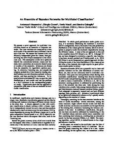
3 Experiment Results Performance Comparison on Gene Data Set
We use two datasets in our experiments. The first dataset is a gene data set and the second dataset is a scene data set. Both datasets are from real world applications and they have natural training data and test data splits. The gene dataset contains 2465 yeast genes and each gene is represented as a 103-dimensional vector [5]. The classification labels are determined using gene functional categories from the Munich Information Center for Protein Sequences Comprehensive Yeast Genome Database(CYGD)2 . The gene dataset is multi-labeled since a gene can have several functions at the same time. In our experiments, we choose 10 base classes and altogether there are 112 different label assignments. The second data set is a scene data set which consists of six base classes which correspond to six different scenes such as beach and sunset etc [1]. These scenes are generally overlapped in the sense that an image can be a member of several classes at the same time. For each image, spatial color moments are used as features and we divide the image into 49 blocks using a 7x7 grid and compute the mean and variance of each band. Each image are then transformed a 49 x 2 x 3 = 294 dimension feature vector. On gene data set, we use the polynomial kernel function of order three, which takes into account pairwise and tertiary correlations among the measurements and is reported to be very efficient [5]. For scene data set, we also use the same kernel function since it produce good results result in our experiments. Figure 1 and Figure 2 present the graphical comparisons on gene and scene data set respectively. Finally, Table 1 and Table 2 present, respectively, the base class performance comparisons of SVM Binary and the meta-learning approach for the two data sets. The base class performance is evaluated using base class precision and recall. From Figure 1 and Figure 2, it is evident that no approach is consistent better than the others across various performance measures. However, we could infer from our study the relationships among various classifiers and measures. For example, SVM binary has the best average precision, coverage, micro-averaged break-even point and recall on both datasets while ADTree has the best micro-averaged precision on both datasets and best one Error and Hamming Loss on gene data set. The study provides empirical evidences for choosing classifiers. Overall, the performances of SVM Binary, ADTree and the meta-learning approach are better than the rest. The results of direct multiclass are the worst. This is largely because in direct multiclass methods, the training data would be fragmented and hence too sparse to build usable models. As we expected, the meta-learning method indeed took the
5 4.5 4
Methods
3.5
ADTree SVM Binary SVM + ADTree C4.8 Binary SVM multiclass C4.8 multiclass
3 2.5 2 1.5 1 0.5
FM
BP
M R
M P
HL Co ve ra ge
AP
On eE rr
Ac cu ra cy
0
Evaluation Measure
Figure 1. Performance Comparisons on Gene Data Set. AP: Average Precision; OneErr: One Error; HL: Hamming Loss; MP: Microaveraged Precision; MR:Mirco-averaged Recall; BP: Micro-averaged Breakeven point; FM: Micro-averaged F1-measure. Performance Comparison on Scene Data Set 1 0.9 0.8
Methods
0.7
ADTree SVM Binary SVM + ADTree C4.8 Binary SVM multiclass C4.8 multiclass
0.6 0.5 0.4 0.3 0.2 0.1
FM
BP
M R
M P
HL Co ve ra ge
AP
On eE rr
Ac cu ra cy
0
Evaluation Measure
Figure 2. Performance Comparisons on Scene Data Set
2 http://mips.gsf.de/proj/yeast/CYGD/db/index.html.
3
advantages of both SVM Binary and ADTree approaches. On gene data set, the meta-learning approach of combining SVM binary and ADTree has smaller one Error and Hamming Loss than SVM Binary and has better Micro-averaged Break-even point and F-measure than ADTree. On Scene data set, the meta-learning approach has the best Hamming loss. It has better Average precision, One error, Mircoaveraged Break-even point and Recall than ADTree and has better hamming loss and micro-averaged precision than SVM Binary. The experimental results of the meta-learning approach confirmed our anticipation. Our study also provides useful insights on the choice of evaluation measures. For rank-based measures, Oneerror only evaluates the top-ranked label while coverage and average precision assess performance on all possible
labels. High coverage usually implies low average precision. Hamming loss takes into account both prediction errors and missing errors. Low one-error usually implies low hamming loss and vice versa. The micro-averaged precision and recall gives equal weight to the samples and thus emphasize larger categories. They are related measures which capture different aspects of the system performance. Microaveraged F1-measure and micro-averaged break-even point combine both precision and recall. They are good measures to use in many situations. The choice of performance measures is crucial in practical applications and the right measure may depend on the problem we faced with. In addition, The Accuracy measure is very aggressive. Note that on gene data set, the accuracy of random guess is 0.0089. On scene data set, the accuracy of random guess is 0.067.
Base SVM Binary SVM+ADTree Class Precision Recall Precision Recall 1 0.678 0.800 0.701 0.760 2 0.952 0.804 0.894 0.678 3 0.743 0.825 0.755 0.755 4 0.818 0.784 0.879 0.674 5 0.473 0.669 0.530 0.528 6 0.529 0.690 0.608 0.570 Table 2. Base Class Performance Comparison on Scene Data Set
4 Conclusion In this paper, we provide a comparative study on various multi-label approaches using both gene and scene data sets. Our study provides useful insights on the relationships among various classifiers as well as various evaluation measures and shed lights on future research. In addition, we propose a meta-learning approach by combining SVM binary approach and ADTree. Our experiments demonstrate that the combine approach could take the advantages of both approaches and is a viable candidate for multi-label problems.
The comparative study also sheds light on the possible research directions. As we mentioned, a potential drawback of the binary approach is the assumption that the categories are conditionally independent from each other, thus ignoring the relation between categories. To consider the dependency among categories, direct multiclass takes the other extreme by transforming multi-label classification problem into multi-class single label classification ones by treating each possible combination of labels as a class. In other words, a ten-label multi-labeled classification problem would be transformed to a 1024-class classification problem. It causes a problem of data sparseness because there are very few examples in certain combination of category labels. The meta-learning approach can be viewed as a comprise as it implicitly consider the correlations among categories using ADTree while taking advantage of the simplicity of binary approach. One of our future work is to build a explicit model for considering the correlation structure between the categories.
Acknowledgments Tao Li is partially supported by a IBM Faculty Research Award, and the National Science Foundation CAREER Award under grant no. NSF IIS-0546280.
References [1] M. Boutell, J. Luo, X. Shen, and J. Luo. Learning multi-label scene classification. Pattern Recognition, 37(9):1757–1771, 2004. [2] A. Elisseeff and J. Weston. A kernel method for multi-labelled classification. In NIPS 14, 2001. [3] T. Joachims. Text categorization with support vector machines: learning with many relevant features. In ECML-98, pages 137–142, 1998. [4] A. McCallum. Multi-label text classification with a mixture model trained by em. In AAAI’99 Workshop on Text Learning, 1999. [5] P. Pavlidis, J. Weston, J. Cai, and W. N. Grundy. Gene functional classification from heterogeneous data. In RECOMB 2001), pages 249–255. 2001. [6] R. E. Schapire and Y. Singer. Boostexter: A boostingbased system for text categorization. Machine Learning, 39(2/3):135–168, 2000. [7] B. Scholkopf and A. J.Smola. Learning with Kernels. The MIT Press, 2002. [8] F. Sebastiani. Machine learning in automated text categorization. ACM Comput. Surv., 34(1):1–47, 2002.
Base SVM Binary SVM+ADTree Class Precision Recall Precision Recall 1 0.557 0.503 0.500 0.562 2 0.743 0.829 0.739 0.773 3 0.363 0.656 0.512 0.468 4 0.480 0.361 0.480 0.440 5 0.482 0.376 0.477 0.447 6 0.634 0.406 0.660 0.547 7 0.506 0.336 0.428 0.418 8 0.405 0.124 0.327 0.273 9 0.477 0.193 0.378 0.257 10 0.353 0.132 0.279 0.209 Table 1. Base Class Performance Comparison on Gene Data Set
4