{km68,feng,sayan,mike}@stat.duke.edu. Abstract. Kernel models have been used extensively in machine learning due to their flex- ibility as non-parametric ...
Empirical Study of a Bayesian Kernel Model Kai Mao, Feng Liang, Sayan Mukherjee, and Mike West Duke University and University of Illinois at Urbana-Champaign Durham, NC and Urbana-Champaign, IL {km68,feng,sayan,mike}@stat.duke.edu
Abstract Kernel models have been used extensively in machine learning due to their flexibility as non-parametric models. Recently a fully Bayesian framework and theory for kernel regression and classification was developed. Models developed in this framework allow for the incorporation of variable selection and other kernel hyper-parameters. This paper is an empirical study of the performance and modeling considerations of this family of models. We first illustrate the efficacy of the model as a point estimator for a variety of simulated and real data. The true benefit of the Bayesian model – estimates and formal modeling of uncertainty – is examined by simulating the posterior distributions of predictions as well the posterior distributions on the relevance of input variables. We will discuss the sensitivity of the posterior to both priors on model parameters and hyperparameters.
1 Introduction Kernel models for regression and classification have been used extensively in machine learning [9, 16, 11, 12]. The appeal of these models are their predictive accuracy, flexibility, and simple extension to high-dimensional data analysis. In the case of certain kernels they are universal approximators [3] and can thus approximate any square integrable function – the basis for non-parametric modeling. The basic formulation of kernel methods is a penalized loss functional [3] � � fˆ = arg min L(f, data) + λkf k2K , f ∈H
(1)
where L is a loss function, H is often an infinite-dimensional reproducing kernel Hilbert space (RKHS), kf k2K is the norm of a function in this space, and λ is a tuning parameter chosen to balance the trade-off between fitting errors and the smoothness of the function. The data are input-output pairs {(xi , yi )}ni=1 with x ∈ Rp and y ∈ {0, 1}, for classification. Due to the representer theorem [4] the solution of the penalized loss functional will be a kernel ˆ = f(x)
n X
wi K(x, xi ),
(2)
i=1
where {xi }ni=1 are the n observed input or explanatory variables.
A Bayesian formulation for kernel methods would provide a natural framework to further the richness and interpretability of kernel models – a program driving much research in data mining and machine learning. Crucially it would provide a formal model of uncertainty and allow for the inference of a full posterior rather than a point estimator. Bayesian versions of kernel models, in particular Bayesian SVMs, have been proposed before [15, 1, 14]. Here the Bayesian analysis is applied on the finite representation from equation (2). This direct adoption of (2) is not a proper model from a Bayesian perspective since the model changes with the sample size without a coherent argument. 1
A fully Bayesian framework and theory for kernel regression and classification addressing the above issues and specifying priors over the entire RKHS was developed in [5]. This model also allowed for variable or feature selection by placing hyperparameters on the kernel. In this paper we provide a careful empirical study of this method and discuss modeling issues such as sensitivity to the priors and uncertainty in the posterior estimates. The summary of this analysis is that our model performs as well or better that well studied and popular methods such as SVMs but provide a formal measure of uncertainty.
2 The Bayesian kernel model In this section we specify the model developed in [5]. The most common approach to putting priors over a RKHS is through the duality between RKHS and Gaussian processes [7, 17]. We do not pursue this approach due to theoretical reasons. The RKHS induced by this approach is larger than the one corresponding to the kernel k. See [5, 8] for detailed discussions. In [5] the space of functions used in modeling is defined as a convolution of the kernel with a signed (Borel) measure � � Z G=
f | f (x) =
k(x, u) dγ(u), γ ∈ Γ ,
(3)
with Γ(·) as a subset of the space of signed Borel measures. Placing a prior on Γ implies a prior on G. An equivalence between G and H exists for an appropriate choice of the the prior distribution on Γ [8]. The prior specified in [5] is such a choice. The model in (3) can be rewritten as Z Z f (x) = k(x, u) dγ(u) = k(x, u) w(u) dF (u),
(4)
where the random signed measure γ(u) is modeled by a random probability distribution F (u) and random coefficients w(u) and F (u) and γ(u) share the same support. In [5] it is assumed that F = FX , the marginal distribution of X, and a Dirichilet Process (DP) prior, DP(α, F 0 ), is used to model uncertainty about the distribution function F . A result of the conjugacy of the DP prior and marginalization over the posterior distribution is that given data Xn = (x1 , ..., xn ) " Z # n X −1 E[f | Xn ] = (α + n) α k(x, u) w(u) dF0 (u) + w(xi ) k(x, xi ) , i=1
taking the limit α → 0, an uninformative prior, the above takes the same form as (2) derived via the i) representer theorem with wi = w(x n . This results the following classification model zi = f (xi ) + ε = w0 +
n X
wj k(xi , xj ) + ε
for i = 1, ..., n,
(5)
j=1
where ε ∼ No(0, 1) and zi is a latent variable that is related to yi by a probit link function, P(yi = 1) = Φ(zi ), with Φ(·) being the standard normal distribution function. To allow for variable or features selection a scale parameter is added for each coordinate in the kernel [2] √ √ kρ (x, u) = k( ρ ⊗ x, ρ ⊗ u)
where a ⊗ b is the element-wise product of two vectors and ρ = (ρ1 , ..., ρp ) is a p-dimensional vector with ρk ∈ [0, ∞]. For the linear and Gaussian kernels the paramterization is kρ (x, u) =
p X
ρ k xk u k ,
k=1
kρ (x, u) = exp − 2
p X k=1
ρk (xk − uk )
2
!
.
The likelihood for the model is n Y
i=1
Φ(zi )yi (1 − Φ(zi ))1−yi .
The hierarchical prior involves a decomposition of the kernel, K = F ∆F 0 . A result of the decomposition is a reparameterization of the regression into the orthogonal factors, F with Kw = F β. We now state our prior specifications w0 ρj τj
∼ Unif(R), βj ∼ No(0, τj ), j = 1, · · · , m ∼ (1 − γ)δ0 + γ Gamma(aρ , aρ s), j = 1, · · · , p � � a τ bτ ∼ InvGamma , s ∼ Exp(as ), γ ∼ Beta(aγ , bγ ) , 2 2
aρ , as , aγ , bγ , aτ , bτ are all hyperparameters that are prespecified. Due to numerical stability not all n factors are included in the decomposition of the kernel matrix resulting in the parameter m < n. The posterior is simulated based on a Markov chain Monte Carlo (MCMC) analysis. A novel MCMC methodology was developed in [5] that added Metropolis-Hastings steps appropriately to deal with the fact that the complete conditionals were not of standard forms. The MetropolisHastings steps were required to update the scale parameters for each coordinate, ρ. The empirical studies will examine predictive accuracy via draws from the posterior. Given a (d) new input x∗ we provide posterior probabilities of its label y ∗ = 1 as Φ(z ∗(d) ) = Φ(w0 + Pn (d) (d) (d) ∗ ∗(d) , w0 , ρ(d) , wj } are samples d = 1, ..., D from the j=1 kρ(d) (x , xj )wj ), where {z Markov chain. Note that for different draws the kernel matrix changes since ρ changes. The other focus of this paper is to study variable selection which will be done by drawing posterior samples of ρ. The Bayesian kernel model will be termed BAKER.
3 Experiments The following experiments on real and simulated data provide an indication of the accuracy of BAKER as a point estimator, a reflection of the uncertainty in the point estimates, and the efficacy and uncertainty in variable selection. 3.1 High-dimensional gene expression data – uncertainty in predictions We first consider a high-dimensional gene expression data set. The purpose of this analysis is to compare the BAKER to an extensively used classifier, the SVM. This example also highlights the utility of the model uncertainty inherent in Bayesian methods. In this example we do not include the variable selection scale parameters to the model. The data set [10, 6] consists of 280 samples from patients of which 190 are tumor samples and 90 are normal. For each sample expression data from 16063 genes and ESTs was collected. The data was randomly split into training and test sets with 180 and 100 samples respectively. A linear kernel was used for both BAKER and SVM with accuracy over twenty random test-train splits of 97.2 ± 1.0% (training) and 88.3 ± 4.1% (test) for BAKER and 98.9 ± .5% (training) and 91.3 ± 2.8% (test) for SVM. The true utility of BAKER is that it provides a predictive distribution and not just a point estimate. We illustrate this on one random test-train split where the test error was 13%. In Figure (1) we plot the mean of the posterior distribution for each test sample in red and provide a point-wise 90% credible interval for each test sample. A result of this analysis is that in addition to misclassified instances there are 7 correctly classified samples with great uncertainty (credible intervals covering 0.5) that may require further investigation. 3.2 Simulated nonlinear classification – variable selection A data set was generated to illustrate the variable selection aspect of BAKER. The data is perfectly separable by a nonlinear classifier and has two relevant dimensions and ten noise dimensions. 3
Predictive Intervals
1 0.9 0.8
Posterior Prob
0.7 0.6 0.5 0.4 0.3 0.2 0.1 0
0
20
40
Instances
60
80
100
Figure 1: The posterior predictive distribution for a test set with the first 10 samples are normal and the remaining tumor. The red stars represent the posterior means and the blue lines are 90% credible intervals. There are 13 cases that are misclassified and 7 more that are very uncertain. Samples from class 0 were drawn from (x1 , x2 ) = (r sin(θ), r cos(θ)), where r ∼ Unif[0, 1] and θ ∼ Unif[0, 2π], xj
∼ Unif[−2, 2], for j = 3, . . . , 12.
Samples from class 1 were drawn from
(x1 , x2 ) = (r sin(θ), r cos(θ)), where r ∼ Unif[1, 2] and θ ∼ Unif[0, 2π], xj
∼ Unif[−2, 2], for j = 3, . . . , 12.
The first two dimensions are signal with class 1 contained in the unit circle and class 0 contained in an annulus outside the unit circle. A draw of the first two dimensions of the data is shown in Figure (2a) We drew 100 training and 100 test samples, 50 for each class. A Gaussian kernel was used and the empirical training and test errors were 0% and 3%, respectively. Posterior means of the precision parameters ρ and the prediction on the region [−2, 2]×[−2, 2] for the first two dimensions are shown in Figure (2b,c). The posterior means for ρ1 and ρ2 are significantly larger than those of dimension 3 to 12 as expected. The prediction on the whole region is accurate. The boundary is approximately the unit circle, the optimal separating boundary. 3.3 UCI Data sets We further examine variable selection and the predictive posterior distribution on several data sets from the UCI Machine Learning Repository1. 3.3.1 Wisconsin Breast Cancer Dataset The Wisconsin Breast Cancer data was examined in [18] using a variety of classifiers. The class labels were benign and malignant and after removal of samples with missing attributes 353 samples remained. The input data had nine attributes. The best result reported in [18] with a training set of 200 samples with 100 from each class and the remaining samples as test was 93.7% by 1 nearest neighbor. We repeated this comparison using BAKER, SVM, and a Generalized Linear Model (GLM) with a probit link as the classification algorithms over ten random 200-153 training-test splits. The classifiers perform comparably: 96.0 ± 1.2% (train) and 95.2 ± .9% (test) for Baker; 96.0 ± .9% (train) and 95.6 ± 1.7% (test) for SVM; 96.0 ± 1.2% (train) and 94.7 ± 1.3% (test) for GLM. 1
ftp://ftp.ics.uci.edu/pub/machine-learning-databases/
4
The Simulated Data
2.5
Posterior Means for ρ
1.4
2
Prediction on the Whole Region
1
−2
0.9
1.2
0.8
1.5
−1
1
0.7
Dim2
1
0.6
0.8
0.5
0 0
0.5
0.6
0.4
−0.5 0.4
0.2 0.2
−1.5 −2 −3
0.3
1
−1
−2
−1
0 Dim1
1
2
3
0
0.1
1
2
(a)
3
4
5
6
7
8
2 −2
9 10 11 12
(b)
−1
0
1
2
(c)
Figure 2: (a) The first two dimensions of the data. Points from class 1 are red stars and points from class 0 are blue circles. (b) The posterior means for all ρ, the signal dimensions are large. (c) The mean posterior probability over all points in the first two dimensions, [−2, 2] × [2, 2]. The posterior predictive distribution for each sample in the test set is displayed in Figure 3. BAKER incorrectly classifies 8 samples 7 of which are benign. However, the 95% credible intervals for each sample indicate that the uncertainty of some of the patients is much larger than that for some others. The credible intervals for a few incorrectly classified samples do not cover 0.5. It would be interesting to look more carefully at these samples, especially sample 8 which has very low posterior probability. Predictive Intervals
1 0.9 0.8
Posterior Prob
0.7 0.6 0.5 0.4 0.3 0.2 0.1 0
0
20
40
60
80 Instances
100
120
140
160
Figure 3: Posterior predictive probabilitys for belonging to the benign class for 153 test samples. The blue line segements represent 95% credible intervals and the red star is the posterior mean. The first 88 samples are benign and the remaining 65 are malignant. All 9 attributes seem relevant as reflected by the posterior means in Figure 4. The second variable “Uniformity of Cell Size” and the ninth variable “Mitoses” seem to be weaker than the others. 3.3.2 Johns Hopkins University Ionosphere database The ionosphere data was examined in [13] using a variety of neural networks. The class labels were good and bad. The input data had 34 attributes. They used the first 200 samples which included 100 bad and good samples as the training set and tested on the remaining 151 samples. They achieved test accuracies of 90.7% by a linear perceptron, 92% by a nonlinear perceptron and 96% by their 5
Boxplot for ρ
8
7
6
ρ
5
4
3
2
1
0
1
2
3
4
5 Dimension
6
7
8
9
Figure 4: Boxplots of the posterior distribution of the the nine values of ρ. implementation of backprop. We repeated this comparison using BAKER and SVM with a Gaussian kernel. The classifiers perform comparably: 97.5 ± .9% (train) and 95.0 ± 1.9% (test) for Baker; 98.9 ± .4% (train) and 96.0 ± 1.1% (test) for SVM.
The posterior predictive distribution on the test set as well as the posteriors for the relevance of each variable are plotted in Figure 5. Classifier is accurate on the test set but the uncertainty for some of the test samples is considerable. Variables 5, 9, 14, 23 have larger relative values and hence should be more significant. Predictive Intervals
1
Posterior Prob
0.8 0.6 0.4 0.2 0
0
50
100
Instances
150
Boxplot for ρ
1.5
ρ
1
0.5
0
5
10
15
Dimension
20
25
30
Figure 5: (a) The posterior predictive probability of a sample being good on the test samples. The first 125 samples are good and the remaining 75 are bad. Red stars are posterior means and blue lines are 95% credible intervals. (b) A boxplot showing the relevant significance for the explanatory variables.
6
4 Modeling considerations The two most important considerations in Bayesian modeling are the computational efficiency of sampling from the posterior and the sensitivity of the posterior to prior specifications. We first consider efficiency. The issue is the amount of time required to obtain coverage of the posterior distribution. The majority of time in the MCMC algorithm is in recomputing the kernel matrix for a new draw of ρ and the computation of the kernel decomposition. For example, a typical run on the Wisconsin Breast Cancer dataset with 1, 000 iterations takes 153.00 seconds in which 91.2% or 139.54 seconds are spent on recomputing and decomposing the kernel (CPU: Intel Xeon 2×2.8GHz; Memory: 4096M; Matlab). This is the computational cost for feature selection. The sensitivity of the posterior to prior specifications is another important issue. We have observed for the model without variable selection the posterior is relatively insensitive to the hyperparameters. For the model with variable selection hyperparameters have an effect on the posterior distribution of relevance for each variable, ρ. However, the prediction is robust with respect to the hyperparameters. In the model with variable selection the two considerations are the probability that a ρ is zero or not and the magnitude of a nonzero ρ. The parameter γ models the prior probability of a variable being relevant reflected by a Beta distribution. We use aγ = bγ = 5 to reflect a prior assumption of half the variables being relevant and the magnitude reflects some degree of concentration. Other values are also possible, but generally do not significantly influence the prediction. The posterior on the ρ values is more sensitive to prior specifications. This is due to the Gamma distribution draws from which can be very large. One possibility to address this is to use a truncated Gamma distribution. Another approach is to examine the hyperparameters that control the tail of the Gamma distribution. The prior magnitude of ρ depends on s which in turn depends on a s . We examine the effect of as on the posterior by running the model setting as = 0.5, 1, 5. The comparisons are run on the Wisconsin Breast Cancer data set. The predictions are robust for all three settings, for example, we examine the first explanatory variable in the first instance of the test set. Figure (6) provides a boxplot of ρ 1 for the three settings of as . It is apparent that the posterior means of ρ1 is very stable however the variance of the posterior distribution of ρ1 is not. As as increases very large values of ρ1 appear in the posterior distribution. These outliers drive the uncertainty in ρ. It is very important to consider this hyperparameter when we model the uncertainty of variable relevance.
5 Discussion We provide a careful empirical examination of a fully Bayesian framework and theory for kernel regression and classification, BAKER, that also allows for variable selection. A conclusion of this study is that BAKER performs comparably well as classifiers such as SVMs while providing a formal measure of model uncertainty. The importance of an estimate of this uncertainty is illustrated on a variety of data sets. The accuracy and models of uncertainty for variable selection is also examined. Lastly we study the priors in the model to better understand setting hyper-parameters.
References [1] S. Chakraborty, M. Ghosh, and B. Mallick. Bayesian non-linear regression for large p small n problems. Preprint is available at http://www.stat.ufl.edu/ schakrab/svmregression.pdf, 2005. [2] O. Chapelle, V. Vapnik, O. Bousquet, and S. Mukherjee. Choosing multiple parameters for support vector machines. Machine Learning, 46(1-3):131–159, 2002. [3] T. Evgeniou, M. Pontil, and T. Poggio. Regularization Networks and Support Vector Machines. Advances in Computational Mathematics, 13:1–50, 2000. [4] G. Kimeldorf and G. Wahba. A correspondence between Bayesian estimation on stochastic processes and smoothing by splines. Ann. Math. Statist., 41(2):495–502, 1971. [5] F. Liang, K. Mao, M. Liao, S. Mukherjee, and M. West. Non-parametric bayesian kernel models. ISDS Discussion Paper Series 2007-10, Duke University, Institute of Statistics and Decision Sciences, 2007. http://ftp.stat.duke.edu/WorkingPapers/07-10.html. [6] S. Mukherjee, P. Tamayo, S. Rogers, R. Rifkin, A. Engle, C. Campbell, T. Golub, and J. Mesirov. Estimating dataset size requirements for classifying DNA Microarray data. Journal of Computational Biology, 10:119–143, 2003.
7
Boxplot for ρ 50 40
ρ
30 20 10 0
0.5
1 a
5
s
Boxplot for Posterior Probabilities
Posterior Prob
1 0.9 0.8 0.7 0.6 0.5 0.5
1 as
5
Figure 6: Boxplots for the posterior draws for ρ1 (upper panel) and the posterior probability of the first benign sample under different hyperparameter values of a s . The predictions shown are similar, but the distribution of ρ1 differs greatly due to outliers under larger as values. [7] E. Parzen. Probability density functionals and reproducing kernel Hilbert spaces. In M. Rosenblatt, editor, Proceedings of the Symposium on Time Series Analysis, pages 155–169. Wiley, New York, 1963. [8] N. Pillai, Q. Wu, F. Liang, S. Mukherjee, and R. Wolpert. Characterizing the function space for Bayesian kernel models. ISDS Discussion Paper Series 2006-18, Duke University, Institute of Statistics and Decision Sciences, 2006. http://ftp.stat.duke.edu/WorkingPapers/06-18.html. [9] T. Poggio and F. Girosi. Regularization algorithms for learning that are equivalent to multilayer networks. Science, 247:978–982, 1990. [10] S. Ramaswamy, P. Tamayo, R. Rifkin, S. Mukherjee, C. Yeang, M. Angelo, C. Ladd, M. Reich, E. Latulippe, J. Mesirov, T. Poggio, W. Gerald, M. Loda, E. Lander, and T. Golub. Multiclass cancer diagnosis using tumor gene expression signatures. Proceedings of the National Academy of Sciences U.S.A., 98:149–54, 2001. [11] B. Sch¨olkopf and A. J. Smola. Learning with Kernels: Support vector machines, regularization, optimization, and beyond. The MIT Press, Cambridge, 2001. [12] J. Shawe-Taylor and N. Cristianini. Kernel Methods for Pattern Analysis. Cambridge Univ. Press, Cambridge, 2004. [13] V. Sigillito, S. Wing, L. Hutton, and K. Baker. Classification of radar returns from the ionosphere using neural networks. Technical Report 10, Johns Hopkins APL Technical Digest, 1989. [14] P. Sollich. Bayesian methods for support vector machines: Evidence and predictive class probabilities. Machine Learning, 46:21–52, 2002. [15] M. E. Tipping. Sparse Bayesian learning and the relevance vector machine. J. Mach. Learn. Res., 1:211– 244, 2001. [16] V. Vapnik. Statistical Learning Theory. Wiley, New York, 1998. [17] G. Wahba. Spline models for observational data. SIAM, Philadelphia, 1990. [18] J. Zhang. Selecting typical instances in instance-based learning. In Proceedings of the Ninth International Machine Learning Conference, pages 470–479. Morgan Kaufmann Publishers, San Francisco, 1992.
8