Towards a Bayesian Statistical Model for the Classification of Causes of Data Loss. Phillip M. Dickens. Department of Computer Science. University of Maine.
Towards a Bayesian Statistical Model for the Classification of Causes of Data Loss Phillip M. Dickens Department of Computer Science University of Maine and Jeffery H. Peden Department of Mathematics and Computer Science Longwood University ABSTRACT Given the critical nature of communications in computational Grids it is important to develop efficient, intelligent, and adaptive communication mechanisms. An important milestone on that path is the development of classification mechanisms that can distinguish between causes of data loss in cluster and Grid environments. In this paper, we investigate one promising approach to developing such classification mechanisms based on the analysis of what may be termed packet-loss signatures that describe the patterns of packet loss in the current transmission window. We analyze these signatures using complexity theory to learn about their underlying structure (or lack thereof), and are mapping the relationship between the complexity metrics and the system conditions responsible for their generation. We show that complexity measures are an excellent metric upon which a classification mechanism can be built. Further, we show how such a classification mechanism can be built based on the application of Bayesian statistics. Introduction Computational Grids create large-scale distributed systems by connecting geographically distributed computational and data-storage facilities via high-performance networks. Such systems, which can harness and bring to bear tremendous computational resources on a single large-scale problem, are becoming an increasingly important component of the national computational infrastructure. At the heart of such systems is the high-performance communication infrastructure that allows the geographically distributed computational elements to function as a single (and tightly-coupled) computational platform. Given the importance of Grid technologies to the scientific community, research projects aimed at making the
communication system more efficient, intelligent, and adaptive are both timely and critical. An important milestone on the path to such next-generation communication systems is the development of a classification mechanism that can distinguish between causes of data loss in current cluster/Grid environments. The idea is to use the classification mechanism to respond to data loss in a way that is appropriate for the particular set of system dynamics responsible for generating such loss. Given this capability, the communication system can take full advantage of the underlying bandwidth when system conditions permit, can back off in response to observed (or predicted) contention within the network, and can accurately distinguish between these two situations. This research is addressing the issue of identifying the root cause(s) of data loss as observed by a high-performance data transfer system during the course of its execution. The approach we are pursuing is to analyze what may be termed packet-loss signatures, which show the distribution (or pattern) of those packets that successfully traversed the end-to-end transmission path and those that did not. These signatures are collected by the receiver and delivered to the sender upon request. Thus the packet-loss signatures are essentially large selective-acknowledgment packets, and are so named based on a growing set of experimental results [14, 15] showing that different classes of error mechanisms have different “signatures”. We are applying complexity theory to the problem of learning the underlying structure (or lack thereof) of these signatures, and mapping the relationship between such underlying structure and the system conditions responsible for its generation. Our research has shown that complexity measures capture quite well the underlying system dynamics, and that understanding such dynamics provides
significant insight into the cause(s) of observed data loss. The test-bed for this research is FOBS1: a high-performance data transfer system for computational Grids developed by the primary author [9-12, 25]. FOBS is a UDP-based data transfer system that provides reliability through a selective-acknowledgment and retransmission mechanism. As noted above, it is precisely the information contained within the selectiveacknowledgment packets that is collected and analyzed by our classification mechanism. Three important factors, whose combination is unique among high-performance data transfer mechanisms for computational Grids, make FOBS an excellent test-bed for this research. First, FOBS is an application-level protocol. Thus the congestion-control mechanism can collect, synthesize, and leverage information from a higher-level view than is possible when operating at the kernel level. Second, the complexity measures can be obtained as a function of a constant sending rate. Thus the values of the variables collected are (largely) unaffected by the behavior of the algorithm itself. Third, FOBS is structured as a feedback control system. Thus the external data (e.g., the complexity measures) can be analyzed at each control point, and this data can be used to determine the duration of the next control interval and the rate at which data will be placed onto the network during this interval. We do not discuss further the design, implementation, or performance of FOBS here. The interested reader is directed to [11-13] for detailed discussions on these issues. In this paper, we focus on distinguishing between contention for network resources and contention for CPU resources. This distinction is important for two reasons. First, contention for CPU cycles can be a major contributor to packet loss in UDP-based protocols such as FOBS. This happens, for example, when the receiver’s socket-buffer becomes full, additional data bound for the receiver arrives at the host, and the receiver is switched out and thus unavailable to pull such packets off of the network. To illustrate this issue, consider a data transfer with a sending rate of one gigabit per second and a packet size of 1024 bytes. Given this scenario, a packet will arrive at the receiving host every 7.9 microseconds, which is approximately the amount of time required to perform a context switch on the
1
Fast Object-Based data transfer System
TeraGrid systems [1] used in this research (as measured by Lmbench [19]). The second reason this distinction is important is that data loss resulting from CPU contention is completely outside of the network domain and should not be interpreted as a growing network condition. This opens the door for new, less aggressive responses, for this class of data loss. It is important to point out that we used contention at the NIC as a proxy for network contention for two reasons: First, while it was relatively easy to create contention at the NIC level, it was extremely difficult to create contention within the 40 gigabit per second networks that connect the facilities on the TeraGrid. Second, we have collected empirical evidence supporting the idea that, at least in some cases, the complexity measures taken from intermediate gigabit routers (from different networks) are quite similar to those measured at the NIC [14]. However, the buffer size and queuing algorithms at intermediate network elements will determine the characteristics of packet loss signatures. This is an important issue, and is the focus of current research. This paper makes two primary contributions. First, it provides significant experimental data showing that complexity measures are quite good at differentiating between causes of packet loss (or at least for those causes that were studied). This shows that there is (at least) one metric that can be used as the basis of a highly accurate classification mechanism. Second, this research studies the statistical characteristics of complexity measures as a function of the cause of loss and the loss rate. It provides empirical evidence (strongly) suggesting that there are as-yet-unknown mathematical properties governing the behavior of complexity measures. This observation is strengthened by the development of simple models that fit the observed data very well. Also, we show that the behavior of complexity values is such that a sophisticated probability model for the causes of packet loss can be developed through the application of Bayesian statistics. Its implementation and evaluation will be the focus of future papers. The rest of the paper is organized as follows. In Section 2, we discuss related research efforts. In Section 3, we describe our diagnostic methodology in the derivation of complexity measures. In Section 4, we describe the experimental design. In Section 5, we present the experimental results. In Section 6, we discuss the
application of Bayesian statistics to the problem of determining the probability that a given cause of data loss is dominant in the light of currently observed complexity measures. In Section 7, we provide our conclusions. 2
Related Work
The issue of distinguishing between causes of data loss has received significant attention within the context of TCP for hybrid wired/wireless networks (e.g., [3-6, 18, 24]). The idea is to distinguish between losses caused by network congestion and losses caused by errors in the wireless link, and to trigger TCP’s aggressive congestion control mechanisms only in the case of congestion-induced losses. This ability to classify the root cause of data loss, and to respond accordingly, has been shown to improve the performance of TCP in this network environment [3, 18, 23]. These classification schemes are based largely on simple statistics on observed round-trip times, observed throughput, or the inter-arrival time between ACK packets [5, 7, 18]. Debate remains, however as to how well techniques based on such simple statistics can classify loss [18]. Another approach being pursued is the use of Hidden Markov Models where the states are characterized by the mean and standard deviation of the distribution of round-trip times [18]. Hidden Markov Models have also been used to model network channel losses and to make inferences about the state of the channel [20]. Our research has similar goals, although we are developing a finer-grained classification system to distinguish between contention at the NIC, contention in the network, and contention for CPU resources. Also, complexity measures of packet-loss signatures appear to be a more robust classifier than (for example) statistics on round-trip times, and could be substituted for such statistics within the mathematical frameworks established in these related works. Similar to the projects discussed above, we separate the issue of classification of root cause(s) of data loss from the issue of implementing responses based on such knowledge. Research into other application-level alternatives to TCP is also related (e.g., [2, 21, 22]). However, none of these projects attempt to determine the root cause(s) of observed packet loss that is a major focus of our research.
3 Diagnostic Methodology The packet-loss signatures can be analyzed as time series data with the objective of identifying diagnostics that may be used to characterize causes of packet loss. A desirable attribute of a diagnostic is that it can describe the dynamical structure of the time series. The approach we are taking is the application of symbolic dynamics techniques, which have been developed by the nonlinear dynamics community and are highly appropriate for time series of discrete data. As discussed below, this approach to classifying causes of packet loss works because of the differing timescales over which such losses occur. In symbolic dynamics [17], the packet-loss signature is a sequence of symbols drawn from a finite discrete set, which in our case is two symbols: 1 and 0. One diagnostic that quantifies the amount of structure in the sequence is complexity. There are numerous ways to quantify complexity. In this discussion, we have chosen the hierarchical approach of d’Alessandro and Politi [8], which has been applied with success to quantify the complexity and predictability of time series of hourly precipitation data [16]. The approach of d’Alessandro and Politi is to view the stream of 1s and 0s as a language and focus on subsequences (or words) of length n in the limit of increasing values of n (i.e., increasing word length). First-order complexity, denoted by C1, is a measure of the richness of the language’s vocabulary and represents the asymptotic growth rate of the number of admissible words of fixed length n occurring within the string as n becomes large. The number of admissible words of length n, denoted by Na(n), is simply a count of the number of distinct words of length n found in the given sequence. For example, the string 0010100 has Na(1) = 2 (0,1), Na(2) = 3 (00,01,10), Na(3) = 4 (001, 010, 101, 100). The first-order complexity (C1) is defined as C1 =
lim (log2 Na(n)) / n .
n − >∞
(1)
The first-order complexity metric characterizes the level of randomness or periodicity in a string of symbols. A string consisting of only one symbol will have one admissible word for each value of n, and will thus have a value of C1=0. A purely random string will, in the limit, have a value of C1=1. A string that is comprised of a
periodic sequence, or one comprising only a few periodic sequences, will tend to have low values of C1. As noted, a hierarchy of complexity values is defined in [8]. The next level of the hierarchy is a quantity termed C2 that captures the fact that random strings are of lower complexity than strings that have rules governing their creation. We do not discuss this quantity here because we have not yet integrated it into our classification mechanism. 3.1 Rational for Complexity Measures Complexity measures work because of the different timescales at which loss events occur. In the case of contention for CPU cycles, packets will start being dropped when the data receiver is switched out and its data buffer becomes full. This is clearly not an issue with TCP, but is an important issue for UDP-based mechanisms. Once the data buffer becomes full, a string of packets will be lost until the receiver regains control of the CPU and is able to pull packets off of the network. The amount of time a receiver is switched out will be on the order of the timeslice of a higher-priority process for which it has been preempted, or the aggregate time-slice of the processes ahead of it in the run queue. Such events are measured in milliseconds, where, as discussed above, the packet-arrival rate is on the order of microseconds. Thus if contention for CPU cycles is the predominant cause of data loss, the packet-loss signatures will consist of strings of 0’s created when the receiver is switched out, followed by strings of 1’s when it is executing. Thus the packet-loss signature will be periodic and will have a low complexity measure. Different operating systems will have different scheduling policies and time-slices, but the basic periodic nature of the events will not change. Data loss caused by contention at the NIC however operates on a much smaller timescale, that being the precise order in which the bitstreams of competing packets arrive at and are serviced by the hardware. The packet-loss signatures represent those particular packets that successfully competed for NIC resources and those that did not. This is an inherently random process, and this fact is reflected in the packetloss signatures. An important question is whether contention at the NIC sheds any light on the packet-loss signatures that are generated by collisions at intermediate routers in the transmission path.
This is obviously dependent on the particular queuing discipline of each router. However, routers that employ a Random Early Detection (RED) policy can be expected to produce packetloss signatures very similar to those produced by contention at the NIC. This is because once the average queue length surpasses a given threshold, the router begins to drop (or mark) packets, and the particular packets to be dropped are chosen randomly. Also, and as discussed above, we have developed a small set of experimental results showing that packet-loss signatures caused by contention at (at least a small set) of intermediate routers are largely equivalent to those observed with contention at the NIC [14]. This is not to say however that the aggregate policies of a large set of intermediate routers will not produce packet-loss signatures that will be misinterpreted by the classification mechanism. This is an important issue and is the focus of current research. 4
Experimental Design
All experiments were conducted on the TeraGrid [1]: a high-performance computational Grid that connects various supercomputing facilities via networks operating at speeds up to 40 gigabits per second. The two facilities used in these experiments were the Center for Advanced Computing Research (CACR, located at the California Institute of Technology), and the National Center for Supercomputing Applications (NCSA, located at the University of Illinois, Urbana). The host platform at both facilities were IA-64 Linux clusters where each compute node consisted of dual Intel Itanium2 processors. The compute nodes at CACR were 1.3 GHz and those at NCSA were 1.5 GHz. The operating system at CACR was Linux 2.4.19SMP, while the operating system at NCSA was Linux 2.4.21-SMP. Each compute node had a gigabit Ethernet connection to the TeraGrid network. The experiments were designed to capture a large set of complexity measures under known conditions. In one set of experiments, the data receiver executed on a dedicated processor within CACR, and additional compute-bound processes were spawned on this same processor to create CPU contention. As the number of additional processes was increased, the amount of time the data receiver was switched out similarly increased. Thus there was a direct relationship between CPU load and the resulting packet loss rate. To investigate loss patterns
5
Experimental Results
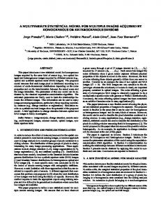
Figure 1 shows the complexity values associated with contention for NIC resources at each data bin. As can be seen, there is a very strong relationship between complexity measures and loss rates. This figure also shows that complexity measures, and the inherent randomness in the system they represent, increases very quickly with increasing loss rate. It can also be observed that the distribution of complexity measures at
each data bin appear to be tightly packed around the mean. As shown in Figure 2, the behavior of complexity measures associated with contention for CPU resources show little change with increasing loss rates. While the distribution of complexity measures in each bin is not as tightly packed as that of contention at the NIC, the measures do appear to be spread out evenly around the mean. Figure 3 shows the mean complexity measures at each data bin with 95% confidence intervals for both causes of data loss. As can be seen, there is a very clear separation of complexity measures even at very low loss rates. In fact, the confidence intervals do not overlap at all for loss rates greater than 0.3%. These are very encouraging results, and provide strong support for the claim that complexity measures are excellent metrics upon which a sophisticated classification mechanism can be built. The development of such a mechanism is considered in the following sections. Complexity Measures: Contention at the NIC
Complexity Measures
0.800
0.700
0.600
Complexity Measures
0.500
0.400 0.000
0.025
0.050
0.075
0.100
Loss Rate
Figure 1. This figure show the complexity measures associated with contention for NIC resources as a function of the loss rate. Complexity Measures: Contention at the CPU 0.600
Complexity Measures
caused by contention for NIC resources, we initiated a second (background) data transfer. The data sender of the background transfer executed on a different node within the NCSA cluster, and sent UDP packets to the node on which the data receiver was executing (there was not a receiver for the background transfer). Initially, the combined sending rate was set to the maximum speed of the NIC (one gigabit per second), and contention for NIC resources was increased by increasing the sending rate of the background transfer. The packet loss experienced by both data transfers was a function of the combined sending rate, and this rate was also set to provide a wide range of loss rates. In all cases the primary data transfer had a sending rate of 1 gigabit per second. In both sets of experiments, the complexity values were computed at each control point. All experiments were performed late at night when there was observed to be little (if any) network contention. We attempted to keep the loss rate within a range of 0 – 10% and to gather a large number of samples within that range. In the case of contention at the NIC, we collected approximately 3500 samples in this range (each of which represented a data transfer of 100 Megabytes). The scheduler made it more difficult to keep the loss rate within the desired range when looking at CPU contention because we had no control over how it switched processes between the two CPUs after they were spawned. This resulted in approximately 1500 samples within the chosen range. For reasons related to the development of the Bayesian analysis (discussed below), we needed to have a large sample of complexity values at discrete (and small) intervals within the loss range. To accomplish this, we sorted the data by loss rate, and binned the data with 30 complexity measures per bin. The bins were labeled with the mean loss rate of the 30 samples.
Complexity Measures
0.525
0.450
0.375
0.300 0.000
0.025
0.050
0.075
0.100
Loss Rate
Figure 2. This figure shows the complexity measures associated with contention for CPU resources as a function of loss rate.
Complexity Measures as a Function of Loss Rate
Complexity Measures
0.800
0.700 Contention at NIC Contention at CPU
0.600
0.500
0.400 0.000
0.025
0.050
0.075
0.100
Loss Rate
Figure 3. The figure shows the mean complexity measure and 95% confidence intervals around the mean as a function of the cause of data loss and the loss rate. 6
Statistical Analysis
(K = KNIC) or ( K
= K CPU ). P(K) is the
probability of cause K occurring, and P(c) is the probability that value c of metric C is observed. In the Bayesian approach, the experimenter’s prior knowledge of the phenomenon being studied is included in prior distributions. In this case, we are able to develop models for P (c | K ) (that is, the likelihood of observing metric C = c given cause K), and the distribution for P(c). Also, P(K) can be set during experimentation since the causes of packet loss are created by the experimenter. We begin by looking at the densities of complexity measures for P (c | K = K CPU ) and P(c | K = K CPU ). 6.1 Data Models
The goal towards which we are working is the development of statistical models that can be used accurately to classify the causes of data loss as the data transfer is progressing. Similar to the approach taken in [18], the classification mechanism will be based on the application of Bayesian statistics. This approach centers on how values of a certain metric – for example, first-order complexity values – can identify a cause of packet loss. We denote the cause of packet loss by K, and consider two cases: the cause of loss is related to contention at the NIC (K = KNIC) or contention at the CPU ( K = K CPU ). (As noted above, we are using NIC contention as a proxy for network contention. A detailed study of contention at intermediate routers under various queuing disciplines is the focus of current research.) Denoting the complexity metric by C, Bayes’ rule states
The behavior of complexity measures appears to be governed by some as-yet-unknown set of mathematical processes. This suggests that it may be possible to develop simple empirical models to describe the distributions for P(c | K = K CPU ) and P(c | K = K CPU ). The approach we used was to feed the complexity measures through a sophisticated statistical program with very powerful tools for fitting models to observed data. Given the shape of the curve for complexity measures associated with NIC contention, it seemed reasonable to investigate models involving exponentials. We tested many models (including polynomial), and the best fit for the data was obtained using the sum of two exponentials. The complexity measures and the model are shown in Figure 4. Sum of Two Exponentials
(1)
Here P ( K | c) is the posterior probability of K given complexity value C = c. That is, it represents the probability of a given cause of data loss in light of the current data (i.e., complexity metric). P (c | K ) is the conditional probability that the value c for metric C is observed when the cause K is dominant. It represents the likelihood of observing complexity measure C = c assuming the model
Complexity Measures
0.800
P (c | K ) ⋅ P ( K ) P( K | c) = P (c )
0.700
Complexity Measures Fitted Data Model
0.600
0.500
0.400 0.000
0.025
0.050
0.075
0.100
Loss Rate
Figure 4. This figure shows the fitted data model when the cause of loss is contention for NIC resources. Figure 5 shows the empirically derived mean complexity measures and 95% confidence intervals, and how they lay on the fitted data model. Visually, it appears to be an excellent fit.
Best Fit Degree 0 Polynomial: Contention for CPU Sum of Two Exponentials
0.700
Mean Complexity Measures and 95% CI Fitted Data Model
0.600
0.600
Complexity Measures
Complexity Measures
0.800
Mean Complexity Measures with 95% CI Best Fit Polynomial 95% Confidence Intervals for Best Fit
0.525
0.450
0.375
0.500
0.300 0.000
0.400
0.025
0.050
0.075
0.100
Loss Rate 0.000
0.025
0.050
0.075
0.100
Loss Rate
Figure 5. This figure shows the mean complexity measures and 95% confidence intervals around the mean and how they lay along the fitted model.
Figure 7. This figure shows the mean complexity measures and 95% confidence intervals around the mean, and how they lay across the fitted data model.
Based on the behavior of complexity measures associated with contention for CPU resources, it appeared that a straight line would provide the best fit for the data. Extensive testing showed this to be true, and Figure 6 shows the fitted data model and the distribution of complexity measures around the model. Figure 7 shows the means and 95% confidence intervals for the empirically derived complexity measures and how they lay along the fitted data model.
6.2 Goodness of Fit.
Best Fit Degree 0 Polynomial: Contention for CPU
Complexity Measures
0.600 Complexity Measures Best Fit Polynomial 95% Confidence Intervals
0.525
0.450
0.375
0.300 0.000
0.025
0.050
0.075
0.100
Loss Rate
Figure 6. This figure shows the fitted data model when the loss is caused by contention for CPU resources.
Visually, it appears that the models describe the empirical data quite well, but more than a visual “match” is required. To construct a model to fit data, there are several criteria that need to be satisfied. Factors such as largest relative residual, the mean relative residual, the sum of the squared residuals, the percentage of residuals greater than a chosen value, and the correlation coefficient should be considered. The analysis of residuals for the two data models is shown in Table 1. As can be seen, the largest relative residual for both models is approximately 14%, while the mean relative residual is 1.37% for the NIC model and 2.58% for the CPU model. The sum of squared relative residuals is particularly good for both models, especially considering the number of data points. The number of data values above and below the theoretical prediction is very close for both data models. The correlation coefficient for the NIC model is excellent. These results indicate a very good fit for both models.
Metric
NIC
CPU
1. LRR: 2. MRR: 3. SSQ: 4. CC: 5. NRA: 6. NRB: 7. RR 10-20% 8. RR 20-80%
13.32% 1.37% 0.447 0.987 1615 1782 0.12% 0%
13.92% 2.58% 0.156 0 772 709 0.81% 0%
1. Largest relative residual 2. Mean relative residual 3. Sum of the squared relative residuals 4. Correlation coefficient 5. Total number of residuals above the theoretical prediction 6. Total number of residuals below the theoretical prediction 7. Relative Residuals in range of 10-20%. 8. Relative Residuals in range of 20-80%.
Table 1. This table shows the metrics used to determine goodness of fit for both fitted data models. 6.3 Distribution of Complexity Measures The empirically derived models fit the data quite well and we will use these as our starting point. The approach is to use the fitted data model as the mean complexity measure at each loss rate. Now the distribution of complexity measures around this mean must be derived. Our working hypothesis is that the data values are normally distributed around the mean of the empirical data. We go about justifying this working conclusion as follows. The obvious first step is to try and rule out a Normal distribution by checking to see if the distribution is clearly non-Normal, and this is clearly not the case. The distribution is not obviously uniform random, for example, because the data clearly cluster quite closely around the mean value, and quickly become more sparsely grouped the farther they are from the mean; in fact, this is a characteristic one would expect of a Normal distribution. The next step is to try to rule out a Normal distribution by testing the numbers of data points contained within the various standard deviations away from the mean. This does not allow us to
rule out a Normal distribution, either. However, so far, all this allows us to conclude is that we cannot easily rule out a Normal distribution. The next step is to perform a hypothesis test using a statistical test for Normality. The one we have chosen is the Shapiro-Wilks test statistic. We applied this test to the data in each data bin, and when outliers were removed from the data, we were, without exception, not required to reject our hypothesis. Based on this, we accept our working hypothesis that this distribution is Normal. 6.4
Use of the Theoretical Model
We now have models for the P( c | K = K CPU ), the P(c | K = KNIC) and, by extension, the P (c)*. Also, we have a working hypothesis that the complexity measures are normally distributed around the mean, and we have a good estimate of the standard deviation around the mean based on the empirical data. We use these models as follows. First, the classification mechanism computes the complexity measure for the current transmission window. Second, we use the fitted data models to find the “theoretical” mean of the complexity measure, at that given loss rate, for each model. The standard deviation around both means is that derived from the empirical data. Next, and given the working hypothesis that the complexity measures are normally distributed about the mean, we are able to compute the likelihood of the complexity measure assuming each model. We do this as follows. For each complexity value xC we compute the distance
xC − µ C from the “theoretical” mean. We then standardize this distance by using the standard deviation so that we have an equivalent distance in the standard normal distribution equal to
xC − µ C σC
(where
σC
is the empirically
derived standard deviation of our hypothesized Normal distribution). The final step is to calculate the area under the curve between the observed complexity measure and the means of the two distributions. However, since this area approaches zero as the observed value approaches the theoretical mean *
P( c) =
P(c | K = K CPU ) * P ( K = K CPU )
+ P(c | K = KNIC) * P ( K = KNIC ).
µ C , we must subtract this value from 1 to arrive at the desired probability value.
3.
7 Conclusions and Future Research In this paper, we have shown that complexity measures of packet-loss signatures can be highly effective as a classifier for causes of packet loss over a wide range of loss rates. Also, it was shown that the divergence of complexity measures, and thus the ability to discriminate between causes of packet loss, increases rapidly with increasing loss rates. However, for loss rates less than approximately 0.003, it was shown that complexity measures in and of themselves are not powerful enough to discriminate between causes of packet loss. Thus one focus of current research is the identification of other metrics or statistical models that can be effective at very low loss rates. This research has also shown that complexity measures lend themselves quite naturally to the development of simple empirical data models. This opens the door to the development of a sophisticated probability model for causes of packet loss based on the application of Bayesian statistics. We are currently working on the implementation of this model. What this research does not answer is the generality of the empirical models. Based on empirical results obtained for other architectures [14,15], we believe that the significant differences between the distributions of complexity measures for causes of data loss, and the general shape of the distributions, will be consistent. This research also does not answer the question of whether random network events can create complexity measures for which our interpretation is incorrect. Both of these issues are the focus of our current research.
4.
5.
6.
7.
8.
References
1. 2.
The TeraGrid Homepage http://www.http://www.teragrid.org Allcock, W., Bester, J., Breshahan, J., Chervenak, A., Foster, I., Kesselman, C., Meder, S., Nefedova, V., Quesnel, D. and Tuecke, S. Secure, Efficient Data Transport and Replica Management for High-Performance Data_Intensive Computing. In the
9.
10.
Proceedings of IEEE Mass Storage Conference, (2001). Balakrishnan, S., Padmanabhan, V., Seshan, S. and Katz, R. A Comparison of Mechanisms for Improving TCP Performance Over Wireless Links. In IEEE/ACM Transactions of Networking, 5(6). Pages 756-769. 1997. Balakrishnan, S., Seshan, S., Amir, E. and Katz, R. Improving TCP/IP performance over wireless networks. In the Proceedings of ACM MOBICON, (November 1995). Barman, D. and Matta, I. Effectiveness of Loss Labeling in Improving TCP Performance in Wired/Wireless Networks. In the Proceedings of ICNP'2002: The 10th IEEE International Conference on Network Protocols, (Paris, France, November 2002). Biaz, S. and Vaidya, N. Discriminating Congestion Losses from Wireless Losses using InterArrival Times at the Receiver. In the Proceedings of IEEE Symposium ASSET'99, (Richardson, TX, March, 1999). Biaz, S. and Vaidya, N. Performance of TCP Congestion Predictors as Loss Predictors, Texas A&M University, Department of Computer Science Technical Report 98-007, College Station, Texas. D'Alessandro, G. and Politi, A. Hierarchical Approach to Complexity with Applications to Dynamical Systems. In Physical Review Letters, 64 (14). Pages 1609-1612. April, 1990. Dickens, P. FOBS: A Lightweight Communication Protocol for Grid Computing. In the Proceedings of Europar 2003, (2003). Dickens, P. A High Performance File Transfer Mechanism for Grid Computing. In the Proceedings of The 2002 Conference on Parallel and Distributed Processing
11.
12.
13.
14.
15.
16.
Techniques and Applications (PDPTA). (Las Vegas, Nevada, 2002). Dickens, P. and Gropp, B. An Evaluation of Object-Based Data Transfers Across High Performance High Delay Networks. In the Proceedings of the 11th Conference on High Performance Distributed Computing, (Edinburgh, Scotland, 2002). Dickens, P., Gropp, B. and Woodward, P. High Performance Wide Area Data Transfers Over High Performance Networks. In the Proceedings of The 2002 International Workshop on Performance Modeling, Evaluation, and Optimization of Parallel and Distributed Systems., (2002). Dickens, P. and Kannan, V. Application-Level Congestion Control Mechanisms for Large Scale Data Transfers Across Computational Grids. In the Proceedings of The International Conference on High Performance Distributed Computing and Applications, (2003). Dickens, P. and Larson, J. Classifiers for Causes of Data Loss Using Packet-Loss Signatures. In the Proceedings of IEEE Symposium on Cluster Computing and the Grid(ccGrid04), (2004). Dickens, P., Larson, J. and Nicol, D. Diagnostics for Causes of Packet Loss in a High Performance Data Transfer System. In the Proceedings of Proceedings of 2004 IPDPS Conference: the 18th International Parallel and Distributed Processing Symposium, (Santa Fe, New Mexico, 2004). Elsner, J. and Tsonis, A. Complexity and Predictability of Hourly Precipitation. In Journal of the Atmospheric Sciences, 50 ((3)). Pages 400-405. 1993.
17. 18.
19. 20.
21.
22.
23.
24.
25.
Hao, B.-l. Elermentary Symbolic Dynamics and Chaos in Dissipative Systems. World Scientific, 1989. Liu, J., Matta, I. and Crovella, M. End-to-End Inference of Loss Nature in a Hybrid Wired/Wireless Environment. In the Proceedings of Modeling and Optimization in Mobile, Ad Hoc, and Wireless Networks (WiOpt'03), (SophiaAntipolis, France, 2003). The BitMover Homepage. http://www.bitmover.com/lmbench/ Salamatian, K. and Vaton, S. Hidden Markov Modeling for Network Communication Channels. In the Proceedings of ACM SIGMETRICS 2001 / Performance 2001, (Cambridge, Ma, June 2001). Sivakumar, H., Bailey, S. and Grossman, R. PSockets: The Case for Application-level Network Striping for Data Intensive Applications using High Speed Wide Area Networks. In the Proceedings of Super Computing 2000 (SC2000). Sivakumar, H., Mazzucco, M., Zhang, Q. and Grossman, R. Simple Available Bandwidth Utilization Library for High Speed Wide Area Networks. In Submitted to Journal of SuperComputing. Tsaoussids, V. and Matta, I. Open Issues on TCP for Mobile Computing. In Journal of Wirelesss Communications and Mobile Computing- Special Issue on Reliable Transport Protocols for Mobile Computing, 2(1). February, 2002. Vaidya, N. and Biaz, S. Discriminating Congestion Losses from Wireless Losses Using InterArrival Times at the Receiver. In the Proceedings of IEEE Symposium ASSET'99, (March, 1999). Vinkat, R., Dickens, P. and Gropp, B. Efficient Communication Across the Internet in Wide-Area MPI. In the Proceedings of The 2001
International Conference on Parallel and Distributed Processing Techniques and Applications (PDPTA). (Las Vegas, Nevada, 2001).