Empirical Study of Feature Selection Methods in Classification Antonio Ara´uzo-Azofra Area of Project Engineering University of Cordoba, Spain arauzo(at)uco.es
Jos´e M. Ben´ıtez Dept. Computer Science and Artificial Intelligence Universidad de Granada, Spain
[email protected]
Abstract The use of feature selection can improve accuracy, efficiency, applicability and understandability of a learning process and the resulting learner. For this reason, many methods of automatic feature selection have been developed. By using the modularization of feature selection process, this paper evaluates a wide spectrum of these methods and some additional ones created by combination of different search and measure modules. The evaluation identifies the most interesting methods and shows some recommendations about which feature selection method should be used under different conditions.
1
Introduction
The task of a classifier is to use feature vectors to assign the represented object to a category or class [10]. Feature selection help us to focus the attention of a classification algorithm in those features that are the most relevant to predict the class. Although theoretically, if the full statistical distribution were known, using more features could only improve results, in practical learning scenarios it may be better to use a reduced set of features [17]. Sometimes a large number of features in the input of induction algorithms may turn them very inefficient as memory and time consumers, even turning them inapplicable. Besides, irrelevant data may confuse algorithms making them reach false conclusions, and hence producing worse results. Apart from increasing efficiency and applicability of classification algorithms, the costs of data acquisition may also be reduced when a smaller number of features is selected. In addition, the understandability of the results of a classification algorithm may be improved. Because of all those advantages feature selection has attracted much attention within the Machine Learning and Data Mining communities and many methods have been developed. According to the different parts identified in feature selection methods [5, 16, 18], its process can be modular-
ized [2] as shown in figure 1. With this modularization almost every feature selection method can be characterized through the evaluation function and search strategy employed. By combining a set of evaluation functions and search strategies we can develop a map of feature selection. We did an extensive review of literature and gathered the most usual evaluation function as well as search strategies. This led to table 1. Our goal was to carry an extensive and rigorous empirical evaluation of the feature selection methods applied for classification. Several reviews on feature selection can be found in the literature, for example, [5, 20, 21]. However, they are incomplete in the sense that the methods considered do not include every feasible cell on table 1. In addition, the set of classification problems considered is rather limited. Our goal was to include a wide spectrum of problems with varied number of features, classes, instances and nature of the features.
Figure 1. Feature selection process
2
Feature Selection methods for Classification
Our intention when addressing the endeavor stated in this paper was to develop a deep empirical study which could help us to gain some insights regarding the suitability of the different proposals in feature selection. Having modularized the process of feature selection, we can take the two main factors (search and measure) and combine them creating a space of feature selection methods. The resulting combinations are represented in table 1.
3
All the feasible combinations are marked with a tick in the table and were selected for evaluation. Some of these combinations had already been proposed somewhere in the literature. To the best of our knowledge, those proposals have been recognized and a reference is included in the corresponding cell. Whenever no method for the combination has been found, we did created the corresponding method.
With the goal stated in the section above in mind we designed and conducted an extensive and rigorous empirical study, out of which meaningful conclusions may be drawn. In this section we provided a detailed description of the experimental method followed, which certainly was hard work.
GA
LVW
[6]
[3]
Wrapper (using 10 fold cross validation)
[26] Mutual information
Relief based feature set measure (RFSM)
[5, 1] Inconsistent example pairs (IEP)
The number of independent experiments is the number of the possible combinations of the three factors above, with some restrictions due to unacceptable high running time: i) feature selection methods that use complete search methods have been applied only to the data sets with less than 16 features and ii) methods with the wrapper measure has not been applied to the biggest dataset (adult). Every experiment has been performed using 10 fold cross-validation. The result shown is always the average of the 10 folds. To assess the significance of results, statistical tests have been used. Following the methodology recommended by Demsar [7] for this type of comparisons, we have used Friedman and Nemenyi statistical tests. A detailed description of these tests can be found in Zar’s book [28].
[6]
ABB
[6]
SFS
3. Classification problem represented in a data set.
Minimum description length criterion
Symmetrical uncertainty
Rough Set consistency
Inconsistent examples (Liu)
[6]
[27]
[1] Basic consistency
Evaluation function
Exhausti. FOCUS 2
B & B
Consistency
Probabilistic
LVF SBS
2. Learning algorithm that generates the classifier,
Information theory
Sequential
1. Feature selection method, with measure and search method as subfactors,
Distance
Complete
Experimental design
Two are the main measures to be taken into account when evaluating a feature selection method: accuracy and feature reduction. Running time is also an important value to study, however, in this work we focus on accuracy and reduction of the number of features. For every classification task, there are three main factors:
SA
Metaheuristic
TS
3.1
Performance
Search method
Empirical methodology
3.2
Data sets
[1] [6] [5] [26] [27] [3]
We wanted to include in the study a wide range of classification problems. So we looked for problems in publicly available repositories seeking for representative problems in different properties. Finally, we have used 36 data sets. They are listed along with their main properties in table 2:
Table 1. Feature selection methods by search strategy and evaluation function
Unfeasible combinations are crossed in the table. They are not adequate because one of the following: i) basic consistency cannot guide any search (it is just a stop measure), ii) FOCUS2 can only use its own measure, iii) BB, ABB and LVF need monotonic measures, iv) LVW is designed for non-monotonic measures.
• Data set column show the name by which data sets are known. • Ex. is the number of examples (tuples) in the data set. • Feat. is the number of features. 2
• Type of features can be:
• ESL: Elements of Statistical Learning [12].
– Discr., all are discrete.
• Org: Dataset from the Orange web site [9].
– Cont., all are continuous.
• Sgi: Dataset repository from Silicon Graphics [11].
– Mixed, both types of features are present.
• Del: Delve (Data for Evaluating Learning in Valid Experiments) [23]
• Cl. is the number of classes. • Unk. is the number of unknown values in the whole data set. Dataset adult anneal audiology balance-scale breast-cancer bupa car credit echocardiogram horse-colic house-votes84 ionosphere iris labor-neg led24 lenses lung-cancer lymphography mushrooms parity3+3 pima post-operative primary-tumor promoters saheart shuttle-landingcontrol soybean splice tic-tac-toe vehicle vowel wdbc wine yeast yeast-class-RPR zoo
Ex. 32561 898 226 625 286 345 1728 690 131 368 435 351 150 57 1200 24 32 148 8416 500 768 90 339 106 462 253
Feat. 14 38 69 4 9 6 6 15 10 26 16 32 4 16 24 4 56 18 22 12 8 8 17 57 9 6
Type Mixed Mixed Discr. Discr. Mixed Cont. Discr. Mixed Mixed Mixed Discr. Cont. Cont. Mixed Discr. Discr. Discr. Discr. Discr. Discr. Cont. Mixed Discr. Discr. Mixed Discr.
Cl. 2 5 24 3 2 2 4 2 2 2 2 2 3 2 10 3 3 4 2 2 2 3 21 2 2 2
Unk. 4262 22175 319 0 9 0 0 67 101 1927 392 0 0 326 0 0 5 0 2480 0 0 3 225 0 0 0
307 3190 958 846 990 569 178 1484 186 101
35 60 9 18 10 20 13 8 79 16
Discr. Discr. Discr. Cont. Cont. Cont. Cont. Cont. Cont. Discr.
19 3 2 4 11 2 3 10 3 7
712 0 0 0 0 0 0 0 214 0
3.3
Classifiers
In order to estimate the quality of feature selection performed by each method, the selected features are tested in a complete learning scenario of classification problems. The following well known learning methods [10] are considered. These methods have been chosen to cover the categories of methods most used. To set up parameters of classifiers, preliminary experiments with different values were performed on the data sets. As we do not intend to compare learning methods, we just use a reasonable approach to get good results. The tests were done with all data sets using all features. The parameter values which performed better on average were chosen. • Naive-Bayes (Nbayes). Despite its lower performance compared with other classifiers, Naive-Bayes is used in real problems with good results [25] and it can be successfully combined in bagging and boosting strategies. Nevertheless, the main reason why we have included this method is that, due to its simplicity, NaiveBayes establishes a base on the minimal performance that other more elaborated methods should improve on. • k Nearest Neighbors (kNN). This method has been considered as a representant of those methods that use distances in classification. After the preliminary experiments, the value k = 15 was chosen as a value large enough to get good results in all considered data sets. • Classification trees [4] (C45). After testing different classification tree learners with the data sets, C4.5 [24] obtained better or similar results to the other tree learners. Besides, C4.5 is well known and commonly used to evaluate feature selectors. For these reasons, we intend this classifier to represent tree and rule based classifiers in our experiments. • Artificial Neural Networks (ANN). There is a great diversity of ANN [13]. As a representation of ANN in classification we have chosen the well known multilayered perceptron. Preferring the simpler systems, just one hidden layer is used, as this is enough for universal approximation [15]. The number of nodes in the hidden layer is adjusted to each dataset by the simple criterion of taking the average between the number of
Table 2. Data sets All data sets have been taken from one of these sources: • UCI: Classification Dataset repository at the University of California at Irvine, Irvine [14]. 3
inputs and outputs. The network will have one output per class, and the class is decided by the output with the highest value. The training algorithm is standard back-propagation with learning rate of 0.1 and a maximum of 500 learning cycles.
3.4
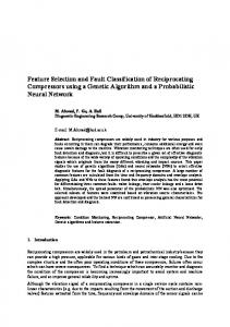
Rows of figure 2 show the results for each of the four considered learning methods. In this way, we can compare the effect of feature selection on each learner and we assure independence for the application of statistical tests. The rectangle shows the Nemenyi critical distance at significance rate of p = 0.05 from the best method. Those methods outside the rectangle can be considered to obtain a worse accuracy.
Data transformations
Some feature selection methods require certain conditions on data. Consequently, data are transformed just for these feature selection methods as described below. After feature selection, original data are passed to the learning methods. For those methods that cannot cope with continuous features these are discretized using equal frequency intervals. More advanced discretization methods [19] were disregarded to avoid collateral effects in feature selection methods. There are methods that only work on continuous features. For those, discrete features were translated to equidistant points in [0, 1]. For those methods that cannot cope with null or unknown values, these values were replaced by the average on continuous features or the most frequent value on discrete features.
3.5
kNN Wra
RFS
Inf RSC IEP
Liu SU
ANN Wra
RSC Liu Inf IEP
MDL
RFS SU
Nbayes Wra
Development and running environment
MDL
RFS
Inf RSC SU IEP Liu
C45 MDL
The software used for learning methods has been Orange component-based data mining software [8], except for artificial neural networks where SNNS [22] was used integrated with OrangeSNNS package. All feature selection methods have been programmed using the Python programming language. Experiments have run on a cluster of 8 nodes with one Xeon Dual 3.2Ghz processor and 1Gb of RAM.
4
MDL
2
3
Wra
RFS
4 Ranking average
Inf RSC Liu IEP
SU
5
6
Figure 2. Comparing accuracy with different relevance measures for SBS search method
Experimental Results Figure 3 shows the same comparison but on the number of features selected. The greater reduction the lower the ranking is. Only the reduction for one learning method is shown (C45). This is because the results are very similar as all measures are independent from the learner except Wrapper. From these two figures we can see how Wrapper and MDL obtain significantly better results than most other measures. However, MDL fails in feature reduction, selecting more features in most cases, while Wrapper show a good compromise being the second in feature reduction. Symmetrical Uncertainty (SU) achieves the greatest reduction, but being the worse on accuracy. It can be concluded that Wrapper is the recommended measure when using Se-
The experiments described took long time to complete and generated a large amount of resulting data. An appropriate summarizing analysis is necessary to interpret them and achieve conclusions. To help in this analysis, many tables and figures have been generated to compare feature selection methods. As an example, figure 2 shows the comparison of relevance measures using ’Sequential Backward Search’. The abscissa axis represents the ranking of each measure in relation with the others. The ranking is in the interval [1, n] when comparing n measures. The lower the ranking the better accuracy was achieved. The value shown for each measure is the average over the 36 data sets. 4
with no significance and SU leads on reduction followed by Wrapper, with significant differences with other methods in most cases. Comparing search methods with each measure, we have not found statistically significant differences. However, SFS leads accuracy on all measures but Wrapper. This is quite interesting because this is a simple and efficient method. Using the Wrapper measure the best search methods are SBS and Exhaustive. Mutual information (Inf) is a commonly used relevance measure in feature selection. As in the other measures, SFS leads accuracy but with no significative difference. Figure 4 shows the comparison according to feature reduction. GA can be rejected because of lower feature reduction while the other methods do not show significative difference for this measure.
No.features SU
Liu
Wra
RSC IEP
RFS
Inf
2
4
3
MDL
5
6
7
Ranking average
Figure 3. Comparing number of features with different relevance measures for SBS search method
quential Backward Search (SBS). Unfortunately, we can not simply deduce that the wrapper approach is the final solution as its main drawback is that its running time may be quite long. It is necessary to point out that precisely on SBS the first set of features to evaluate is the complete set —which includes all of them. And this may imply too long a time for a wrapper solution. If results among learners are compared, we can see how in C45 results are more similar for all measures than within other learners. As this is a general observation on other figures, it may be concluded that feature selection influences C45 less than other learners. Intuitively, we can think that the reason is that C45 has its own feature selection embedded.
No.features TS
2
3
ABB
4
Ex BB LVF
GA SFS
5 Ranking average
SA
SBS 6
Figure 5. Convex hull grouped by type of search method with results of C4.5
7
To provide a global view of results, as showing all methods in one figure will not be clear, their convex hulls are drawn instead. Figure 5 shows the convex hulls for the ranking results obtained with all methods for the C4.5 learner. Each convex hull is computed out of the ranking results for the feature selection algorithms grouped by its type of search method. In this type of plots, the best methods would be near the origin of both axis since this means better accuracy and simultaneously higher feature reduction. In figure 5, we can see the contraposition of accuracy versus feature reduction as methods with better accuracy get worse reduction and vice versa It is not a surprise that complete search group has the nearest frontier to origin. As these methods explore all feature sets, this is the expected result when evaluation func-
Figure 4. Comparing number of features with different search methods for mutual information relevance measure
Comparing measures with other search methods, the following facts can be observed. On complete searchbased methods, despite not finding significant differences —probably because only 21 data sets could be used— , Wrapper stands out with better accuracy and reduction when exhaustive search is used. On those complete searchbased methods that require monotonic measures, Liu and Information Gain leads to better results. Using Sequential Forward Search (SFS) we have not found significant differences on accuracy but IEP stands out on reduction. On randomized search methods, Wrapper leads on accuracy 5
tions provide appropriate information. Nevertheless, sequential search group has achieved pretty near results while having a better efficiency, that allows them being applied to much more data sets. Because of the position of probabilistic and metaheuristic groups, we can see they have achieved worse results, specially on accuracy. Maybe the reason is that they need more iterations, more time than the other methods to get similar results. On the other hand, the advantage of these methods is that, in most cases, they can improve the results attained as more running time is allowed.
5
[6] M. Dash and H. Liu. Consistency-based search in feature selection. Artificial Intelligence, 151(1-2):155–176, 2003. [7] J. Demsar. Statistical comparisons of classifiers over multiple data sets. Journal of Machine Learning Research, 7:1– 30, 2006. [8] J. Demsar and B. Zupan. Orange: From experimental machine learning to interactive data mining. (White paper) http://www.ailab.si/orange, 2004. [9] J. Demsar, B. Zupan, and G. Leban. Datasets. http://www.ailab.si/orange/datasets.asp, 2006. [10] R. O. Duda, P. E. Hart, and D. G. Stork. Pattern Classification. Wiley-Interscience, 2nd edition, 2001. [11] S. Graphics. Datasets. http://www.sgi.com/tech/mlc/db/, 2006. [12] T. Hastie, R. Tibshirani, and J. Friedman. The Elements of Statistical Learning: Data Mining, Inference, and Prediction. Springer-Verlag, New York, 2001. [13] S. Haykin. Neural Networks. A comprehensive foundation. Prentice-Hall, 1999. [14] S. Hettich and S. D. Bay. The uci kdd archive. http://kdd.ics.uci.edu/, 1999. [15] K. Hornik, M. Stinchcombe, and H. White. Multilayer feedforward networks are universal approximators. Neural Networks, 2:359–366, 1989. [16] A. Jain and D. Zongker. Feature selection: Evaluation, application and small sample performance. IEEE Trans. Pattern Analysis and Machine Intelligence, 19(2):153–158, February 1997. [17] R. Kohavi and G. H. John. Wrappers for feature subset selection. Artificial Intelligence, 97(1-2):273–324, 1997. [18] P. Langley. Selection of relevant features in machine learning. In Procedings of the AAAI Fall Symposium on Relevance, pages 1–5, New Orleans, LA, USA, 1994. AAAI Press. [19] H. Liu, F. Hussain, C. L. Tan, and M. Dash. Discretization: An enabling technique. Data Mining and Knowledge Discovery, 6:393–423, 2002. [20] H. Liu and H. Motoda. Feature Selection for Knowledge Discovery and Data Mining. Springer, 1998. [21] H. Liu and L. Yu. Toward integrating feature selection algorithms for classification and clustering. IEEE Transactions on Knowledge and Data Engineering, 17(3), March 2005. [22] U. of Stuttgart. Stuttgart neural network simulator. http://www-ra.informatik.uni-tuebingen.de/SNNS/, 1995. [23] U. of Toronto. Data for evaluating learning in valid experiments. http://www.cs.utoronto.ca/˜delve/, 2003. [24] J. R. Quinlan. C4.5: Programs for Machine Learning. Morgan Kaufmann, 1993. [25] I. Rish. An empirical study of the naive bayes classifier. In IJCAI 2001 Workshop on Empirical Methods in Artificial Intelligence, 2001. [26] P. Scanlon, G. Potamianos, V. Libal, and S. M. Chu. Mutual information based visual feature selection for lipreading. In Int. Conf. on Spoken Language Processing, South Korea, 2004. [27] J. Sheinvald, B. Dom, and W. Niblack. A modelling approach to feature selection. In 10th International Conference on Pattern Recognition, volume i, pages 535–539, 1990. [28] J. H. Zar. Biostatistical Analysis. Prentice-Hall, New Jersey (US), 4th edition, 1999.
Conclusions
An extensive and rigorous empirical study on feature selection methods for classification has been presented. To cover the spectrum of the great number of feature selection methods we have created and evaluated new methods by combination of evaluation functions with search strategies. The experiments confirmed the usefulness of feature selection improving results in most of the problems while reducing the number of features used. The suspected contraposition of accuracy and feature reduction is also corroborated. The wrapper approach is confirmed as the best option when it can be applied. In these cases, the recommended search strategy is Exhaustive or SBS. When wrapper is not applicable the results suggest using consistency measures or information gain. To achieve higher feature reduction the IEP measure can be used with SFS search. These are only some recommendations that may be extracted from the empirical study. Applying some data mining or rule extraction techniques may lead us to an expert system that assist in finding the best method to use for each feature selection problem. As the results vary through learning methods, in future work it may be interesting to study the tolerance to irrelevant features of each learning method.
References [1] H. Almuallim and T. Dietterich. Learning boolean concepts in the presence of many irrelevant features. Artificial Intelligence, 69(1-2):279–305, 1994. [2] A. Arauzo-Azofra, , J. M. Benitez, and J. L. Castro. Consistency measures for feature selection. Journal of Intelligent Information Systems, 2008. [3] A. Arauzo-Azofra, J. M. Benitez, and J. L. Castro. A feature set measure based on relief. In Proceedings of the fifth international conference on Recent Advances in Soft Computing, pages 104–109, Nottingham, UK, December 2004. [4] L. Breiman, editor. Classification and regression trees. Chapman & Hall, 1998. [5] M. Dash and H. Liu. Feature selection for classification. Intelligent Data Analysis, 1(1-4):131–156, 1997.
6