Feature Selection and Extraction for Malware Classification

JOURNAL OF INFORMATION SCIENCE AND ENGINEERING 31, 965-992 (2015)

Feature Selection and Extraction for Malware Classification CHIH-TA LIN1, NAI-JIAN WANG1, HAN XIAO2 AND CLAUDIA ECKERT2 1 Department of Electrical Engineering National Taiwan University of Science and Technology Taipei, 106 Taiwan E-mail: {d9507932; njwang}@mail.ntust.edu.tw 2 Chair for IT Security, Institute of Informatics Technischen Universität München Garching, 85748 Germany E-mail: {xiaoh; claudia.eckert}@in.tum.de

The explosive amount of malware continues their threats in network and operating systems. Signature-based method is widely used for detecting malware. Unfortunately, it is unable to determine variant malware on-the-fly. On the hand, behavior-based method can effectively characterize the behaviors of malware. However, it is time-consuming to train and predict for each specific family of malware. We propose a generic and efficient algorithm to classify malware. Our method combines the selection and the extraction of features, which significantly reduces the dimensionality of features for training and classification. Based on malware behaviors collected from a sandbox environment, our method proceeds in five steps: (a) extracting n-gram feature space data from behavior logs; (b) building a support vector machine (SVM) classifier for malware classification; (c) selecting a subset of features; (d) transforming high-dimensional feature vectors into low-dimensional feature vectors; and (e) selecting models. Experiments were conducted on a real-world data set with 4,288 samples from 9 families, which demonstrated the effectiveness and the efficiency of our approach. Keywords: dynamic malware analysis, data classification, dimensionality reduction, term frequency inverse document frequency, principal component analysis, kernel principal component analysis, support vector machine

1. INTRODUCTION The growth of malicious programs is exponent. Symantec blocked approximately 5.5 billion malware attacks in 2011, yielding an increase greater than 81% compared with 2010. [1] Signature-based antivirus systems are widely used for detecting viruses in real time. However, according to AV-Comparatives statistics [2], commercial products provide a 14%-69% detection rate regarding new malware. Moreover, viruses can be easily manipulated by hackers, producing numerous variants. It is easy to change malware signatures to evade detection by anti-virus software; thus, it is impossible to update the signature database as rapidly as the explosive speed at which malware variants are developed. The behaviors of two given malware variants remain similar, although their signatures may be distinct. Recent studies have developed tools to monitor and analyze malware behaviors [3-12]. Egele [13] surveyed automated dynamic malware analysis techniques and tools; automated dynamic analysis provides a report for each malware program, describing its run-time behavior. The information yielded by these analysis tools Received November 12, 2013; revised June 11 & September 1, 2014; accepted October 11, 2014. Communicated by Shou-De Lin.

965

966

CHIH-TA LIN, NAI-JIAN WANG, HAN XIAO AND CLAUDIA ECKERT

elucidates malware program behaviors, facilitating the timely and appropriate implementation of countermeasures. Rieck [14] analyzed malware behavior by using a CWSandbox environment [12], identifying typical malware families as classified by standard anti-virus software; after examining single-family models by using the machine learning toolbox, a malware behavior classifier was constructed. The Institute for Information Industry (III) developed a sandbox environment to record malware behavior; the sandbox can collect the activity of a file, registry, or process. Compared with signature-based methods, behavior-based methods can improve the accuracy of malware classification. However, the time cost for training a classifier is higher than that of training a signaturebased method. The computational demands of a behavior-based method cannot meet the requirements of a real-world scenario because excessive time is consumed during feature extraction and model adaptation. Bordes [23] proposed a novel online algorithm, namely, LASVM (fast large-scale support vector machine), which can reduce the execution time by 30% when retraining the classifier; however, the time increased in O(n2) with respect to the number of features. To reduce the time cost of behavior-based malware detection, we propose a twostage dimensionality reduction approach, combining feature selection and extraction to substantially reduce the time cost. Malware behavior logs were collected from a sandbox environment, and an n-gram feature data set was generated based on function calls and bag-of-words model. Feature selection and extraction methods were analyzed to reduce the dimensionality of features, and a support vector machine (SVM) method was used to build the classifier. We showed that using term frequency inverse document frequency (TF-IDF), principal component analysis (PCA), and kernel principal component analysis (KPCA) methods can reduce the number of dimensions, maintaining a promising predictive accuracy. In addition, the selected and extracted features reflected the major behaviors of malware families. Moreover, we propose a multigrouping (MG) algorithm to further improve classification in small feature sets. The proposed approach yielded promising performance and efficiency levels.

2. RELATED WORK Dynamic behavior analysis is an effective method for predicting unknown malware. Sun et al. [24] proposed a method for detecting worms and other malware by using sequences of WinAPI calls and depending on fixed API call addresses. Tsyganok et al. [25] proposed a measure of similarity by using system calls to classify the malware. The classification error ranged from approximately 18.5% to 21.4%. Wang et al. [26] used two – to three API function call sequences to describe eight suspicious behaviors. The experiment involved using a Bayes algorithm to classify whether program was malicious and achieved 93.98% when 80% of the data were used to train in 914 samples with 453 malicious malwares. Hegedus et al. [27] proposed random projections and k-nearest neighbor classifiers. By using the proposed methodology as well as the knowledge and experience of an F-Secure Corporation expert, 24 malware candidates were extracted from 2441 original candidates, of which 25% were known to be malicious and 50% were likely to be malicious. Palahan et al. [28] collected 2393 executables from 50 malware families to produce 2393 system call dependency graphs, and achieved an 86.77% accuracy result. Nakazato et al. [29] proposed a classification method that consists of two

FEATURE SELECTION AND EXTRACTION FOR MALWARE CLASSIFICATION

967

primary techniques, namely N-gram and TF-IDF. The frequency of N-gram Windows sequence API log data was extracted from 2312 malware samples. The characteristics of the malware samples were deduced by using the TF-IDF technique. By using TF-IDF scores and call sequences as the cluster algorithm for classification, the average precision and recall were approximately 55% and 90%, respectively. For analysis of a substantial amount of computing, Liu et al. [30] used MapReduce to reduce the overhead time to improve performance by more than 30%. The experimental result regarding accuracy was 45% (from 50% to 90%) for detecting Trojans, viruses, worms, and spyware. The reduction in time cost in this study cannot be achieved if a high number of malwares or features are used in the classifier. Unlike certain studies that have focused on the identification of specific Windows API call sequences, key values, and parameters for malwares, our classifier incorporated a multigrouping (MG) TF-IDF and PCA, and a KPCA algorithm was used to determine the effective API sequences and was combined with the SVM learning algorithm. Determining the most effective API behavior composition for malware families and rebuilding the classifier in a competitive time-saving manner is easy. After conducting feature selection and extraction analysis, we determined the composition and weighting of behavior functions for malware families. Our results were consistent with the general cognition of the major proportion of malware behaviors.

3. METHODOLOGY To perform online malware analysis, the retraining and forecasting of updated malicious behaviors must be completed as rapidly as possible; thus, the number of features must be reduced in the learning and classification step. We exploited the feature selection and extraction techniques, using a support vector machine (SVM) classifier, proposing a generic dimension reduction method to update the learning model in few seconds. The following basic steps outline the proposed learning approach: 1: Behavior monitoring and data preprocessing. A corpus of malware binaries was executed and logs were collected using a sandbox environment based on hardware virtualization technology to avoid anti-malware detection. Regarding the application programming interface (API) function calls, the feature data were generated based on behavior logs by using the bag-of-words model. 2: Training and testing. Machine learning techniques were applied to classify malware families and determine the optimal classifiers and parameters to achieve the ideal accuracy and learning times. 3: Feature selection analysis. The effective feature set was calculated using the TF-IDF algorithm. The feature weighting was determined based on the TF-IDF value to determine which feature set yields the optimal accuracy and learning times. 4: Feature extraction analysis. The reduced feature dataset was converted from term frequency data by using the PCA and KPCA algorithms to determine the optimal reduced feature set that yields the optimal accuracy and learning times. 5: Model selection and online extension. Based on the effective and reduced feature sets, machine learning techniques were applied to classify the malware families; the goal was to determine the optimal classifiers and parameters that yielded the ideal accuracy and learning times.

968


These steps and the corresponding technical details are presented in detail in the subsequent sections. 3.1 Behavior Monitoring and Data Preprocessing The malware behavioral datasets were collected from a sandbox environment based on the hardware virtualization technology developed by the Institute for Information Industry (III). The malware was executed in a guest operation system (Microsoft OS) that started on a host computer operation system (Xen) and communicated with a virtualization layer. The sandbox recorded the behavior function calls from the guest operation system, which include cross-matching data (hidden files, hidden registry, hidden connection), file Activity, registry activity, process activity, and generating a detailed report. Table 1 provides an example of the operations observed in the analysis reports. The report collected up to 150 seconds (approximately 30,000 procedures) of data after the malware was executed. Including the non-malware family programs, 4,288 samples of nine families were executed and recorded. The malware families and numbers of each malware family were shown in Table 2. Table 1. An example of operations as reported by sandbox during run-time analysis. No. Content 1 CALL name: [], cr3: [0xc08e000] pid: [856],tid: [908], NtOpenKey (0x12fc74: 0x0, 0x80000000, 0x12f950: \Registry\Machine\Software\Microsoft\Windows NT\CurrentVersion\Image File Execution Options\Adware.Admedia.exe) ts-2012-02-11_00:23:42; 2 CALL name: [], cr3: [0xc08e000] pid: [856],tid: [908], NtOpenKey (0x12fc74: 0x0, 0x80000000, 0x12f950: \Registry\Machine\Software\Microsoft\Windows NT\CurrentVersion\Image File Execution Options\Adware.Admedia.exe) 3 CALL name: [C:\Adware.Admedia.exe], cr3: [0xc08e000] pid: [856],tid: [908], NtOpenKeyedEvent(0x12fb14: 0x7c99b140, 0x2000000, 0x12faec: \KernelObjects\CritSecOutOfMemoryEvent) ts-2012-02-11_00:23:42; … …

Label 1 2 3 4 5 6 7 8 9 Total

Table 2. The malware families and numbers of each malware family. Number Malware families Sample names Adware 377 Adware.Casino, Adware.Downloader,... Virus/Exploit 76 Exploit.DCOM, Backdoor.Agent,... Dialer 210 Dialer.Riprova, Dialer-110,... Heuristic 348 Heuristic.Trojan, Heuristic.W32,... Suspect.Trojan 129 Suspect.Trojan.Generic,... Trojan 1510 Trojan.Agent, Trojan.Downloader,... W32 207 W32.Luder, W32.Virut,... Worm 1042 Worm.Allaple, Worm.Mydoom,... Non-Malware 389 winlogon.exe, smss.exe,... 4288


969

Most studies of malware dynamic analysis have attempted to clarify the specific feature function sets of family behaviors. Rieck [14] based on the vector space and bagof-words models, finding shared behavioral patterns, and yielding implicit feature set and the vector space data to analysis. For generic purposes, we extracted the function call word for each analysis report, using the bag-of-words model to generate a high-dimensional feature space corpus. A document is characterized by the frequencies of the words it contains. We referred to the set of considered words as feature set F and denoted the set of all analysis reports using D. Given a word   F and a report d  D, we determined the number of occurrences of n in d to calculate the frequency f = (d, ). We derived an extracting function  that maps analysis reports to an |F|-dimensional vector space by considering the frequencies of all words in F.

: D  R|F|, (D)  (f = (d, ))F

(1)

The 4,288 documents yielded 187 distinct words; that is, F contained 187 dimensions in the resulting vector space that corresponded to the frequencies of these words in the analysis reports. The word  was encoded with identifiers that ranged from 1 to 187. Table 3 listed the words and identifier of the corpus dictionary. Table 3. Examples of the words and identifier of the corpus dictionary. Name of words Identifier 1 NtOpenKey 2 NtOpen-KeyedEvent 3 NtQuerySystem-Information 4 NtAllocate-VirtualMemory 5 NtOpen-DirectoryObject 6 NtOpenSymbolic-LinkObject 7 NtQuerySymbolic-LinkObject 8 NtClose 9 NtFsControlFile 10 NtQueryVolumeInformationFile … …

To analysis the effect of consecutive words, the n-gram model was applied in our corpus. The unigram feature space f = (d, ) was equivalent to the bag-of-words model, and the bigram to six-gram feature space were acquired based on the unigram feature space. We assembled the consecutive words N from  in F to form n-gram feature set FN. Given a word N  FN and a report d  D, we determined the number of occurrences of n in d and calculated the frequency fN = (d, N). We derived an extracting function N that maps the analysis reports to an |FN|-dimensional vector space by considering the frequencies of all words in FN:

N: D  R|F |, N(D)  (f = (d, N)) F , N=1,6. N

N

N

The number and examples of n-gram words were shown in Table 4.

(2)


970

Table 4. The number and example of n-gram words. n-gram unigram bigram trigram four-gram five-gram six-gram

Number of distinct word 187 6740 46216 130671 242663 367211

Sample of Word 1, 2, 3, 4, 5, 6, 7, 8, 9, 10, 11, 12, 13, 14, 15, 16, 17, 18, 19, 20, ... 1 1, 1 2, 1 3, 1 4, 1 5, 1 6, 1 7, 1 8, 1 9, 1 10, 1 11, 1 12, 1 13, ... 1 1 1, 1 1 2, 1 1 3, 1 1 4, 1 1 5, 1 1 6, 1 1 7, 1 1 8, 1 1 9, 1 1 10, ... 1 1 1 1, 1 1 1 2, 1 1 1 3, 1 1 1 4, 1 1 1 5, 1 1 1 6, 1 1 1 8, 1 1 1 10, ... 1 1 1 1 1, 1 1 1 1 3, 1 1 1 1 4, 1 1 1 1 5, 1 1 1 1 6, 1 1 1 1 10, ... 1 1 1 1 1 1, 1 1 1 1 1 2, 1 1 1 1 1 3, 1 1 1 1 1 4, 1 1 1 1 1 8, ...

3.2 Training and Testing The n-gram feature space data fN = (d, N) introduced in the previous section can be applied in various learning algorithms. SVMs [15] were originally designed for use in binary classification. Hsu [16] constructed a multiclass classifier by combining several binary classifiers. The training data from the ith and the jth classes in the one-against-one method is required to solve the following binary classification problem: 1

( ij )T ( ij )  C   ij min t  ij ,bij , ij 2 ij T ij ij ( )  ( xt )  b  1  t , if yt  i, t

(3)

( )  ( xt )  b  1   , if yt  j , ij T

ij

ij t

tij  0

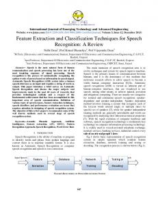
where the training data xt are mapped to a high dimensional space by using the kernel function , the penalty parameter is C, and the  is the normal vector to the hyperplane. If sign (ij)T(xt)+bij indicates it is in the ith class, one is added to the vote for the ith class. Otherwise, the jth is increased by one. Regarding the k class label, k(k1)/2 classifiers must be constructed. The kernel is related to the transform (xi) by the equation k(xi, xj) = (xt)(xt). The SVM effectiveness depends on the kernel selection, the kernel parameters, and soft margin parameter C. The Gaussian radial basis function k(xi, xj) = exp(γ||xi  xj||2) was used to maximize the hyperplane margins. The kernel parameters γ and cost parameters C must be estimated to yield the optimal prediction. The LIBSVM tool [17], which is an established SVM method, was included in the test environment. Fig. 1 shows the process of data training and classification. The new tuning γ and C values are selected using a grid search, first using exponentially growing sequences, and subsequently using a binary search for precision until the accuracy is less than 10-3.

Fig. 1. The process of the data training and classification.


971

3.3 Feature Selection Analysis Learning calculation is extremely time-consuming for high-dimensional datasets. The TF-IDF [18] is a numerical statistic that reflects the importance of words in document collections or corpuses. Jing [19] used the TF-IDF feature selection method to process data resources and establish the vector space model, providing a convenient data structure for text categorization. A typical TF-IDF calculation can be expressed as follows: Wi =TF(i, d)  IDF(i)

(4)

where Wi is the weight of word ωi in document dD, TF(ωi, d) is the term frequency, or the number of ωi in d, and IDF (i )  log(

D DF (i )

)

(5)

where IDF is the inverse document frequency and DF(ωi) represents the appearance of ωi in D. The largest value of IDF(ωi) occurs when ωi appears only in one document and its effect is particularly substantial. To sort the weighting of ωi with all dD, we normalized the sum of term frequency and modified the TF-IDF model as follows:

Wi 

TF (i , dl )  IDF ( ),for all l in D. i max{TF (i , dl )}

(6)

To enhance the accuracy of feature selection, we proposed the following MG TFIDF method:

Wi ,k 

TF ( , d )  IDF max{TF ( , d )} i

l ,k

i ,k

i

, for all l in D and k = 1,9.

(7)

l

The Wi,k was calculated by picking the k-family of malware data, using individualized feature selection for each malware family. ∑TF(ωi, dl,k) is sum of the term frequency of ωi in the kth class. IDFi,k is the modified inverse document frequency for the kth class: '

IDFi,k  10(1IDFk )IDFk

(8)

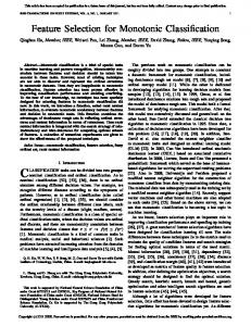
where IDF′k = (IDF(ωi)IDF(ωi,k))/(|D||Dk|), indicates that the exceptive proportion of ωi in the kth class dataset is as small as possible. IDFk = IDF(ωi,k)/|Dk|, indicates that the apparent proportion of ωi in the kth class dataset is as large as possible. Fig. 2 shows the feature selection process. Regarding data learning and classification using the TF-IDF method, the first m features in the Wi sequence were selected to train and classify. The initial γ and C could be chosen from the same values in the feature domain training. We can determine the optimal accuracy by increasing m in the test. Regarding the MG TF-IDF method, the first m features in the Wi,k sequence for all nine families were collected and filtered using the duplicate feature to test.

972


Fig. 2. The process of feature selection.

3.4 Feature Extraction Analysis Feature extraction is a dimension reduction method that reduces the number of random variables being considered. We introduced PCA and KPCA in the feature extraction algorithms to reduce the time cost of learning calculation for high-dimensional datasets. 3.4.1 Principal component analysis The central concept of PCA [20] is reducing the dimensionality of a dataset that comprises numerous interrelated variables, retaining as much variation as possible within the dataset. This is achieved by transforming to a new set of variables, the principal components (PCs), which are uncorrelated and ordered so that the first retain most of the variation present in the original variables. Given a dataset comprising m features (α′1, α′2, …, α′m), the intent is to transform into a new set of p variables (α1, α2, …, αp) of maximal variance. The first step is selecting a linear function α′1ω of the elements of ω that exhibits maximal variance, where α′1 is a vector of p constants α11, α12, …, α1p, denoting transpose, where p

1'  111   122  ...  1 p p  1 j j .

(9)

j1

Next, a linear function α2ω is determined, which is uncorrelated with α′1ω and exhibits maximal variance, and so on, so that at the mth stage a linear function α′mω exhibits a maximal variance subject to being uncorrelated with α′1ω, α′2ω,…, α′m-1ω. To derive the form of the PC, first consider α′1ωi; the vector α′1 maximizes α′1ω = α′1∑1α1. To maximize α′1∑1α1 subject to α′1α1 = 1, the standard approach is using the Lagrange multipliers technique, maximizing as follows:

111  1(11  1)

(10)

where λ1 is a Lagrange multiplier. Differentiation with respect to α1 yields or

11  11 = 0, 11 = 11

(11)

(1  1Ip )1 = 0,

(12)

where Ip is the (p  p) identity matrix. Thus, λ1 is an eigenvalue of ∑1 and α1 is the cor-


973

responding eigenvector. ∑1 is the covariance matrix of feature 1,





T yl 1 ylq

l  1,| D | obeservations of documents

1

|D|

,

(13)

where yl 1  ( f ( d1 , 1 )  (  l 1 y l1 ) /( D ) /  1 is the standard dataset score value as calculated based on the original dataset and σ1 is the standard deviation of 1st feature. The new feature space dataset g was generated as follows: D

gj = yj, j = 1, p

(14)

where the λ value could represent the degree of importance of the new vector, and λ1 > λ2 > λ3> … > λp. To locate the principal component of each malware family, we proposed a MG PCA method, solving the following problem for each kth family class: (k  kIp)k = 0, k = 1, 9.

(15)

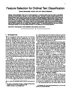
We picked the kth class data from the training dataset and generated the standard score value dataset yk. The new transformation vector k and λk were calculated for each class. We reorganized the new transformation vector , which was chosen using classby-class selection and the λ sorted value. A new MG feature dataset g was generated using gnew = yold. Fig. 3 shows PCA feature extraction process; regarding PCA data learning and classification, the first m features in the new dataset g were selected to train and classify. We can determine the optimal accuracy by increasing and testing m. Regarding the MG PCA method, the first m features of gk in all nine families were collected for testing.

Fig. 3. The process of PCA feature extraction.

3.4.2 Kernel principal component analysis The KPCA is a non-linear extension of the PCA. [21] Its advantages are nonlinearity of eigenvectors and an increased number of eigenvectors. Karg [22] applied PCA, KPCA and linear discriminant analysis to kinematic parameters and analyzed for feature


974

extraction. In PCA, the eigenvalue problem is solved as follows:

  , where  

yyT

D

.

(16)

∑ is a covariance matrix. If we nonlinearly map the data into a feature space F by using a non-linear map  : RN  F, y  Y

(17)

linear PCA is performed in the high-dimensional space F, corresponding to a non-linear PCA in the original data space. The covariance matrix is calculated as follows: l   T C   D l  N . T

(18)

The eigenvalue problem determines Eigenvalues λ ≥ 0 and Eigenvectors VF, satisfying CV = λV, where V = Φ. This yields the following: (T) = (T)N

(19)

thus, the Eigenvalue problem becomes (K  N) = 0 or K = (N), where K = T.

(20)

The scalar product of Φ can be substituted with a kernel function K. In this study, a Gaussian kernel K(xi, xj) = exp(γk||xixj||2) was used. The new feature space dataset g was generated using the following formula: gj 

 Tj K j

,

j  1, p .

(21)

Where λ1 > λ2 > λ3 > … > λp and the λ value could represent the degree of importance of the new vector. To focus on finding the principal component of each malware family, we proposed an MG KPCA method. We solved the problem for each kth family class as follows: (Kk  Nk) = 0, k = 1, 9.

(22)

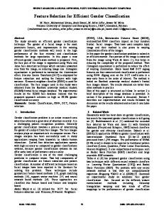
We picked the kth class data from training dataset, generated the standard score value dataset yk, and calculated Kk. The γk in Gaussian kernel K must be tuned to yield the optimal transformation. The new transformation vectors k and λk were calculated for each class. We reorganized the new transformation vector , which was selected classby-class, and by the λ sorted value. The new MG feature dataset g was generated using gnew = TK/. Fig. 4 shows the KPCA feature extraction process, involving data learning and classification. The first m features in new dataset g were selected to train and classify. The optimal values of γk and m were determined using a grid search method in two loops. Regarding the MG KPCA method, the first m features of gk in all nine families were collected to test.


975

Fig. 4. The process of KPCA feature extraction.

3.5 Model Selection and Online Extension The numbers and instances of features are the major time consumers in online machine learning. Bordes [23] proposed a novel online algorithm (LASVM) that converged SVM solutions. The experimental evidence for diverse datasets indicates that the LASVM method reliably reaches competitive accuracy levels after performing a single pass of the training set. The effectiveness of LASVM could reduce the execution time by 30% when regenerating classifiers; the time increased in quadratic complexity (n2-order) as the number of features increased. We propose a novel dimension reduction algorithm to substantially reduce the number of features used in machine learning. Our two-stage dimension reduction algorithm could save more than 99% of execution time during the re-training process of high feature spaces. The proposed algorithm is described as follows: f(d, )  F(f(d, ))  f(d, ), y(d, )  G(y(d, ))  g(d, m)  H(g(d, m))  z(d).

(23)

The first stage F(f(d, ω)) involves using the feature select algorithm detailed in Section 3.3, where f(d, ω′) is the selected subset of the original dataset and y is the standard score value of f. The second stage G(y(d, ω′)) involves using the feature extraction algorithm detailed in Section 3.4, where g(d, m) is the dimension reduction dataset of y and H(g(d, m)) is machine learning process that uses the SVM algorithm detailed in Section 3.2, yielding z(d) as the final prediction of document d to evaluate the accuracy. In practical online application, the parameters in this process should be adjusted to reduce the learning time. The optimal parameters could be determined by using initial offline dataset. We used a 40% training dataset and f(d, ω)→F(f(d, ω))→f(d, ω′)→H(g(d, m))→z(d) to determine the optimal feature subset, and then used Equation (4) to calculate the optimal m and γk for feature reduction, γ and C for SVM. The online training was simulated by initially collecting 40% of a dataset, and the parameters were fixed in the following training and testing. The classifier was rebuilt to accumulate 50% to 90% of the data in increments of 10% and tested for the subsequently incoming 10% of the dataset.

976


4. EXPERIMENT We collected 4,288 documents from nine family classes of malware samples, as described in Section 3.1. Cross validation was used to identify effective parameters, allowing the classifier to accurately predict unknown data and prevent overfitting. [18] In vfold cross-validation, the training set is divided into v subsets of equal size. Sequentially one subset is tested using the classifier trained on the remaining v1 subsets. This is called the holdout method if v = 2. We used three-part cross validation, modifying the v-fold cross-validation to yield an estimate. We generated 10-fold data subsets: four subsets were the training set, one subset was the estimate set used for optimal parameter tuning, and the remaining five subsets were used in independent testing. Total 10 runs were tested by random combination of 10-fold subsets data. A confusion matrix is a specific table layout that displays the performance level of a classification system; thus, a confusion matrix table was generated and the accuracy was evaluated for each estimated subset and testing subset. 4.1 Behavior Monitoring and Data Preprocessing In the first experiment, we examined the general classification performance level of the proposed malware behavior classifier. The learning and classification methods described in Section 3.2 were used to analyze a unigram to six-gram dataset. Various methods were used to evaluate our retrieval system. Table 5 lists the result of families for the first-fold SVM test, using unigram, where TP no. = the number of true positives, FN no. = the number of false negatives, FP no. = the number of false positives, TN no. = the number of true negatives, accuracy A = (TP + TN)/(TP + FN + FP + TN), precision (Sensitivity) P = TP/(TP + FP), recall R = TP/(TP + FN), specificity S = TN/(TN + FP), negative predictive value N = TN/(TN + FN), and F-measure F = 2PR/(P + R). Table 5. Various measures result of families by 1st run SVM test for unigram. Label TP no. FN no. FP no. TN no. A P R S N F 1 184 16 33 1936 0.98 0.85 0.92 0.98 0.99 0.88 2 26 20 12 2111 0.99 0.68 0.57 0.99 0.99 0.62 3 87 11 12 2059 0.99 0.88 0.89 0.99 0.99 0.88 4 123 55 27 1964 0.96 0.82 0.69 0.99 0.97 0.75 5 50 16 23 2080 0.98 0.68 0.76 0.99 0.99 0.72 6 642 90 126 1311 0.9 0.84 0.88 0.91 0.94 0.86 7 57 51 34 2027 0.96 0.63 0.53 0.98 0.98 0.57 8 489 43 44 1593 0.96 0.92 0.92 0.97 0.97 0.92 9 183 26 17 1943 0.98 0.92 0.88 0.99 0.99 0.89

Table 6 lists the results of the 10-run SVM test for the unigram dataset, where 9

9

9

Micro Precision   TPi /( TPi   FPi ) , i 1

i 1

i 1

9

9

9

i 1

i 1

i 1

Micro Recal   TPi /( TPi   FN i ) ,


9

9

i 1

i 1

977

9

Micro Specificity   TN i /( TN i   FPi ) , i 1

9

9

9

i 1

i 1

i 1

Micro Negative predictive value   TN i /( TN i   FN i ) , 9

Macro Precision   Pi / 9 , i 1 9

Macro Precision   Ri / 9 , i 1

9

Macro F   Fi / 9 , i 1

Table 6. The further measures result of families by 10-run SVM test for unigram. Macro Macro nth Run Micro P Micro R Micro S Micro N Macro F Precision Recall 1 0.8488 0.8488 0.9811 0.9811 0.8012 0.7801 0.7885 2 0.8418 0.8418 0.7784 0.7634 0.9802 0.9802 0.7693 3 0.8387 0.8387 0.7908 0.7866 0.9798 0.9798 0.7847 4 0.8413 0.8413 0.7856 0.7678 0.9802 0.9802 0.7743 5 0.8559 0.8559 0.7944 0.8047 0.9820 0.9820 0.7953 6 0.8583 0.8583 0.7827 0.7802 0.9823 0.9823 0.7803 7 0.835 0.835 0.7961 0.758 0.9794 0.9794 0.7703 8 0.8506 0.8506 0.8127 0.7888 0.9813 0.9813 0.7988 9 0.8555 0.8555 0.8152 0.8029 0.9819 0.9819 0.808 10 0.8398 0.8398 0.8033 0.7525 0.9800 0.9800 0.7744 average 0.8466 0.8466 0.9808 0.9808 0.796 0.7785 0.7844

The microprecision and micro recall values were the same for the multiclass classification, and the microspecificity and micronegative predictive values were the same. We observed that all of the micronegative predictive values were higher than 97.9%. The results revealed a satisfactory prediction for the negative predictive value. Therefore, the experiments focused on overall true positives; in other words, the microprecision (and recall) measure was used for assessing accuracy and optimizing the parameters. Figs. 5

(a) Recall (b) Negative predictive value Fig. 5. The confusion result of families for unigram 1strun classify (C = 500, γ = 0.00000093).

978


and 6 show the confusion matrix results and micro measures results of the families in the first-run SVM test for unigram. The matrix diagonal corresponds to the recall value of each class, and the total accuracy was the micro recall value.

(a) Microprecision (= micro recall) (b) Micronegative predictive value Fig. 6. The micro measures result of each family for unigram classify (C = 500, γ = 0.00000093).

(a) Average microprecision w.r.t. N-gram. (b) Time cost w.r.t N-gram. Fig. 7. The microprecision and the time cost of n-gram experiments.

Fig. 7 shows the average microprecision of the used feature numbers and the corresponding time costs of the n-gram experiments. The average values comprised the results of the 10-run experiment. In Fig. 7 (a), the microprecision gradually increased from the unigram to the four-gram experiment, inconspicuously increasing in the five-gram and six-gram experiments; thus, numerous features in the increased five-gram and six-gram experiments were redundant and ineffective. By contrast, in Fig. 7 (b), the time cost continually increased as the size of the feature dimension increased. The time costs of these experiments failed to meet the requirements of online machine learning. 4.2 Feature Selection Analysis In the first experiment, we determined that the time cost of a machine depended on


979

the feature dimension size and most features might be redundant and ineffective. Dimension reduction attempts to reduce the time cost of machine learning. In this experiment, we selected the feature subsets of data by using various selection methods, conducting learning and classification testing as described in Section 3.2. Fig. 8 shows the results of the TF-IDF feature selection method (Section 3.3) as compared with those of the random selection method. The MG TF-IDF feature selection method uses the smallest number of

(a) Unigram

(c) Trigram

(b) Bigram

(d) Four-gram

(e) Five-gram (f) Six-gram Fig. 8. The microprecision results of diverse feature selection methods.

980


features, attaining similar microprecision levels; thus, the MG TF-IDF method precisely selects the effective features of individual malware families and is superior to the TFIDF feature selection method, substantially reducing the required feature dimension, particularly in the proposed MG TF-IDF method, whereby 100-1000 selected features were sufficient to maintain equivalent micro precision. Reducing the feature dimension to less than 1% would allow time cost savings of 99% in high dimensional feature spaces. As shown in Fig. 8, we observed that the accuracy of four-gram, five-gram, and sixgram MG TF-IDF methods exhibited a similar tendency of increasing to nearly the same final best accuracy. The MG TF-IDF method effectively selected the major behaviors of each malware family in the unigram test. Table 7 lists the first 10 major words of unigram selected by MG TF-IDF method for malware families. Table 7. The first 10 selected words of malware families by MG TF-IDF method in unigram test. Adware Virus/Exploit Dialer 1 NtOpenKey NtClose NtWriteFile 2 NtClose NtOpenKey NtReadFile 3 NtQueryValueKey NtQueryValueKey NtClose 4 NtDelayExecution NtSetValueKey NtQueryValueKey 5 NtQueryKey NtCreateKey NtOpenKey 6 NtWaitForSingleObject NtAllocateVirtualMemory NtAllocateVirtualMemory 7 NtQueryInformationToken NtMapViewOfSection NtWaitForSingleObject 8 NtOpenThreadTokenEx NtQueryAttributesFile NtMapViewOfSection 9 NtOpenProcessTokenEx NtProtectVirtualMemory NtQueryAttributesFile 10 NtQueryInformationProcess NtReadVirtualMemory NtRequestWaitReplyPort Heuristic Suspect.Trojan Trojan 1 NtClose NtClose NtClose 2 NtOpenKey NtOpenKey NtQueryAttributesFile 3 NtQueryValueKey NtQueryValueKey NtOpenKey 4 NtQueryVirtualMemory NtMapViewOfSection NtDelayExecution 5 NtOpenFile NtReadVirtualMemory NtQueryDirectoryFile 6 NtQueryInformationProcess NtUnmapViewOfSection NtYieldExecution 7 NtQueryDirectoryFile NtQueryKey NtQueryValueKey 8 NtQueryInformationToken NtWaitForSingleObject NtOpenFile 9 NtAllocateVirtualMemory NtClearEvent NtQueryInformationProcess 10 NtMapViewOfSection NtQueryInformationToken NtMapViewOfSection W32 Worm Non-Malware 1 NtClose NtClose NtClose 2 NtOpenKey NtDelayExecution NtOpenKey 3 NtQueryValueKey NtAllocateVirtualMemory NtQueryValueKey 4 NtMapViewOfSection NtWaitForSingleObject NtWaitForSingleObject 5 NtReadVirtualMemory NtOpenKey NtQueryInformationToken 6 NtQueryAttributesFile NtCreateEvent NtAllocateVirtualMemory 7 NtUnmapViewOfSection NtDeviceIoControlFile NtReleaseMutant 8 NtAllocateVirtualMemory NtQueryValueKey NtMapViewOfSection 9 NtOpenThreadTokenEx NtRequestWaitReplyPort NtQueryDefaultLocale 10 NtOpenProcessTokenEx NtResumeThread NtEnumerateValueKey


981

In addition to the common function, we observed the following:  The behaviors of peeping user preferences of operation appear in the Adware family. (e.g. Query Key Value, Query Information)  The behaviors of installing and launching program by weaknesses of service appear in the Virus/Exploit family. (e.g. SetValueKey, CreateKey, AllocateVirtualMemory)  The behaviors of sending information or files appear in the Dialer family. (e.g. Read/ Write File, WaitForSingleObject, RequestWaitReplyPort)  The behaviors of evading the detection of antivirus system appear in the Heuristic family. (e.g. QueryVirtualMemory, QueryInformationProcess, QueryDirectoryFile)  The behaviors of loading the software into memory appear in the Suspect.Trojan family, e.g. MapViewOfSection, ReadVirtualMemory, UnmapViewOfSection.  The behaviors of launching the task and querying information of files appear in the Trojan family. (e.g. QueryAttributesFile, DelayExecution, QueryDirectoryFile, YieldExecution)  The behaviors of slowing down the operation of the windows system appear in the W32 family. (e.g. QueryValueKey, ReadVirtualMemory, NtOpenThreadTokenEx, NtOpen-ProcessTokenEx)  The behaviors of continuously copying files, installing and executing softwares appear in the Worm family. (e.g. DelayExecution, CreateEvent, DeviceIoControlFile, RequestWaitReplyPort, ResumeThread)  The less maliciou behaviors appear in the Non-Malware family. (e.g. no CreateThread, CreateKey, Read/Write File, AllocateVirtualMemory, DelayExecution) Table A (Appendix A) lists the first 10 major words of further grams that were selected using the MG TF-IDF method for Dialer malware and four-gram tests of Nonmalware. A spyware dialer is a malicious program that attempts to create a connection to the Internet or another computer network over the analog telephone, modem, or Integrated Services Digital Network (ISDN) by using WinAPIs. We observed that a serial of NtWriteFile/NtReadFile words were selected in bi-, tri-, and four-gram test, convinced the major behaviors of a spyware dialer. Besides, we observed that most behaviors in the non-malware were key related operation, were significant differences with malware families. Fig. 9 shows the results of the MG TF-IDF feature selection method from unigram to six-gram. We observed that a high gram yielded favorable accuracy with sufficient words (approximately 1000). If the number of selected features was low (e.g., 10), the accuracy of a high gram was relatively poor. The number of combinations for front ranking function in a high gram was high and accompanied by a low probability. A large number of features caused over-training and resulted in no increase or decrease of test accuracy. In general, the four-gram model demonstrated optimal performance regarding the final accuracy compared with the five-gram model and high gram, and was sufficient for representing the research results of using the most effective selection and parameter tuning method. Besides, five-gram had a 4288242663 big dataset, maybe need to test in Hadoop platform to solve the resource problem. Considering a large amount of memory and an exponential increase in the time cost of a high gram compared with that of the four-gram model, we focused on investigating unigram to four-gram models in practice.

982


Fig. 9. The microprecision results of diverse grams of MG TF-IDF feature selection.

4.3 Feature Extraction Analysis Feature selection is a dimension reduction method that reduces the original mass features. In this experiment, we converted the original feature data into new reduced feature space data by using the feature extraction methods described in Section 3.4, conducting learning and classification testing as described in Section 3.2. The PCA and MG PCA method were used to extract the major behaviors of malware effectively to form few representative components. Table 8 lists the highest five principal component score weightings and the combination of latent functions extracted using the PCA method in the unigram test. Table 8. The highest five principal component score weightings and the combination of latent functions extracted using the PCA method in the unigram test. principal component score weighting 1st 0.242798 2nd 0.181731 3rd 0.126186 4th 0.068949 5th 0.062883 2nd principal component 1st principal component Behavior function Percent contribution Behavior function Percent contribution NtClose 44.17 NtQueryAttributesFile 25.93 NtQueryAttributesFile 14.61 NtReadFile 24.86 NtOpenKey 14.28 NtClose 19.95 NtQueryValueKey 6.01 NtWriteFile 14.27 NtDelayExecution 4.65 NtDelayExecution 10.14 NtOpenFile 3.47 NtOpenFile 6.30 NtQueryInformationProcess 2.29 NtQueryVirtualMemory 6.21 NtAllocateVirtualMemory 2.21 NtQueryInformationProcess 3.73 NtQueryDirectoryFile 2.04 NtReadVirtualMemory 3.70 NtMapViewOfSection 1.35 NtQueryDirectoryFile 3.51


983

We observed the increased operation of the registry key and memory in the first principal component, and the increased operation of files in the second principal component, corresponding to the generic cognition of virus attack characteristics. Table B (Appendix B) lists the first principal component score weighting and the combination of latent functions extracted using the MG PCA method for malware families. The front ranking functions of each family were approaching to the MG TF-IDF observations shown in Table 7. Table C (Appendix C) lists the first principal component and the combination of latent functions for additional grams that were selected using the MG KPCA method for Dialer malware. Fig. 10 shows the results of PCA and KPCA as compared with other feature extraction methods. MG KPCA demonstrated a substantial improvement in prediction accuracy. As Kung [31] mentioned, the kernel approach dealt with the relationship and similarity between training set and test set, the bigram test of MG KPCA method demonstrated a substantial improvement (approximate 95% accuracy) in prediction accuracy. When the number of transformed features was small, the MG KPCA method achieved greater microprecision than did the other feature reduction methods. As few as 10-30 transformed features (i.e., 1-3 PCs selected from each malware group) could sufficiently represent individual characteristics, generating an accurate classification. By contrast, increasing the number of transformed features yielded overfitting and reduced the microprecision levels.

(a) Unigram

(b) Bigram

(c) Trigram d) Four-gram Fig. 10. The microprecision results of diverse feature extraction methods.


984

Although the PCA and KPCA methods can minimize the time cost of the learning and classification processes, it increases the time cost of the feature extraction process. Table 9 shows the time cost for each estimate method. Compared with the training time for the bag-of-words dataset and PCA methods, the MG PCA method reduced the time cost by approximately 25%. The KPCA and MG KPCA methods doubled the time cost; thus, the PCA and MG PCA methods were the most effective at reducing the time cost of online training. Table 9. The time cost (seconds) of 40% dataset training for various procedure. unigram bigram trigram four-gram Bag of word PCA MG PCA KPCA MG KPCA

F.E.

SVM

Total

0.6 1.1 46 33

5.5 1.7 5.3 1.9 2.1

5.5 2.3 6.4 48 35

F.E. SVM Total

F.E.

147 32 1.7 175 6.1 458 3 312 1.5

942 126 2 237 4.6 2849 3.1 2452 1.4

147 34 181 461 314

SVM Total

942 128 242 2852 2453

F.E.

SVM

Total

469 678 6356 5971

3074 1.7 3.2 1.8 1.7

3074 471 681 6358 5973

(Test environment: Quard-Core AMD Opteron(tm) Processor 2384, CPU: 800MHz) (F.E.: The Process of Feature Extraction.)

4.4 Model Selection and Online Extension Feature selection and extraction were verified to reduce time cost. In this experiment, we combined these methods, forming a two-stage dimension reduction method as described in Section 3.5, and conducting learning and classification testing as described in Section 3.2. Online learning was simulated in accumulating 50% to 90% of the data in increments of 10% to train and collected the subsequently incoming 10% of the dataset to test. The first online simulation experiment was comparing the effectiveness between all feature selection and MG TF-IDF feature selected methods. Fig. 11 shows the microprecision level and time cost results; the prediction microprecision value of both methods were highly approaching, however, MG TF-IDF methods saved increasingly more time as the n-gram number increased.

(a) Unigram (b) Bigram Fig. 11. The microprecision level and time cost results of various combination methods.


985

(c) Trigram (d) Four-gram Fig. 11. (Cont’d) The microprecision level and time cost results of various combination methods.

To decrease the time cost, we combined the MG TF-IDF and feature extraction methods, forming a two-stage feature reduction method. Table 10 lists the selected and extracted feature numbers in the experiment. Table 10. The number of selected features and extracted feature of various experiment. unigram bigram trigram four-gram (1) (2) (1) (2) (1) (2) (1) (2) MG TF-IDF + PCA 60 50 1000 50 1000 50 1000 50 MG TF-IDF + MG PCA 60 50 1000 100 1000 100 1000 100 MG TF-IDF + KPCA 60 50 1000 50 1000 50 1000 50 MG TF-IDF + MG KPCA 60 100 1000 100 1000 100 1000 100 (1: no. of selected feature, 2: no. of extracted feature)

Fig. 12 shows the microprecision results of the online training simulation, using various combined methods. With the more data collected, the accuracy had gradually increased. In the bigram to four-gram online simulations, the trends and value of prediction microprecision were highly approaching to the whole selecting features test. The accuracy of our feature selection and reduction approach continued to fit the performance as original whole dataset test.

(a) Unigram (b) Bigram Fig. 12. The microprecision results of various combination methods in online simulation.

986


(c) Trigram (d) Four-gram Fig. 12. (Cont’d) The microprecision results of various combination methods in online simulation.

(a) Unigram

(b) Bigram

(c) Trigram (d) Four-gram Fig. 13. The total time cost results of the online training simulation.

Regarding the time cost analysis, Fig. 13 shows the total time cost results of the online training simulation, using various combined methods. The MG TF-IDF selection algorithm combined with the PCA or MG PCA extraction algorithms yielded the minimal time cost. The accuracy of our feature selection and reduction approach continued to fit the performance as original whole dataset test. The execute time of the rebuilding the classifier was below 10s, the findings show that the proposed algorithm significantly


987

reduces the time cost and meets the online learning requirement of collecting malware behavior every minute.

5. CONCLUSIONS Using high-dimensional n-gramor mapping data space can enhance classification predictions; however, such enhancements cost excessive computing time. The primary contribution of this study is the proposed two-stage feature reduction method, which substantially reduces the time cost of classifying malware behavior by using automatic online learning. The key components of the proposed approach comprise (a) using the MG TF-IDF feature selection method to precisely select the effective features of data subsets in the first stage; (b) using PCA or KPCA to convert the original feature space to a low PC feature space in the second stage; (c) automatically tuning the learning and classification by using learning algorithms; and (d) combining feature selection and extraction with learning and classification, and applying these methods to online detection. The malware behavior log data were collected from a sandbox environment based on hardware virtualization technology. The proposed system executed and recorded 4,288 samples from nine malware families. The dimensionality reduction, TF-IDF, PCA, and KPCA methods were analyzed to reduce the time cost of classification. Furthermore, we proposed an MG algorithm for each feature of the reduction method; the findings showed the effectiveness of its feature reduction. Moreover, we evaluated our method by using an online training simulation experiment. Our two-stage dimensionality reduction approach substantially reduced time costs. Combining the MG TF-IDF, PCA, and SVM methods for online training allows the re-training and classifying procedures to be completed in few seconds, meeting the online learning requirements for collecting malware behavior every minute. The proposed sandbox test environment uses a similar concept as hypervisor architecture that is easily applied to cloud environments. The propose approach offers a competitive malware detection procedure.

APPENDIX A Table A. The first 10 words of Dialer malware selected using the MG TF-IDF method from the bigram to four-gram tests and four-gram tests of Non-malware. bigram trigram 1 NtWriteFile, NtReadFile NtWriteFile, NtReadFile, NtWriteFile 2 NtReadFile, NtWriteFile NtReadFile, NtWriteFile, NtReadFile 3 NtQueryValueKey, NtQueryValueKey NtQueryValueKey, NtQueryValueKey, NtQueryValueKey 4 NtOpenKey, NtOpenKey NtWriteFile, NtWriteFile, NtWriteFile 5 NtOpenKey, NtQueryValueKey NtOpenKey, NtQueryValueKey, NtClose 6 NtWriteFile, NtWriteFile NtQueryInformationToken, NtClose, NtOpenKey 7 NtClose, NtOpenKey NtOpenProcessTokenEx, NtQueryInformationToken, NtClose 8 NtQueryValueKey, NtClose NtOpenThreadTokenEx, NtOpenProcessTokenEx, NtQueryInformationToken 9 NtClose, NtClose NtClose, NtOpenKey, NtQueryValueKey 10 NtFsControlFile, NtWaitNtWaitForSingleObject, NtFsControlFile, NtWaitForSingleObject

ForSingleObject


988

four-gram tests of Dialer malware 1 2 3 4 5 6 7 8 9 10

NtReadFile, NtWriteFile, NtReadFile, NtWriteFile NtWriteFile, NtReadFile, NtWriteFile, NtReadFile NtQueryValueKey, NtQueryValueKey, NtQueryValueKey, NtQueryValueKey NtWriteFile, NtWriteFile, NtWriteFile, NtWriteFile NtOpenThreadTokenEx, NtOpenProcessTokenEx, NtQueryInformationToken, NtClose NtOpenProcessTokenEx, NtQueryInformationToken, NtClose, NtOpenKey NtReadFile, NtReadFile, NtReadFile, NtReadFile NtFsControlFile, NtWaitForSingleObject, NtFsControlFile, NtWaitForSingleObject NtDelayExecution, NtRequestWaitReplyPort, NtDelayExecution, NtRequestWaitReplyPort NtRequestWaitReplyPort, NtDelayExecution, NtRequestWaitReplyPort, NtDelayExecution

1 2 3 4 5 6 7 8 9 10

NtEnumerateValueKey, NtEnumerateValueKey, NtEnumerateValueKey, NtEnumerateValueKey NtQueryValueKey, NtQueryValueKey, NtQueryValueKey, NtQueryValueKey NtOpenThreadTokenEx, NtOpenProcessTokenEx, NtQueryInformationToken, NtClose NtOpenProcessTokenEx, NtQueryInformationToken, NtClose, NtOpenKey NtDuplicateObject, NtQueryValueKey, NtQueryValueKey, NtClose NtQueryKey, NtDuplicateObject, NtQueryValueKey, NtQueryValueKey NtEnumerateKey, NtOpenKey, NtEnumerateKey, NtOpenKey NtClose, NtClose, NtQueryKey, NtDuplicateObject NtOpenKey, NtEnumerateKey, NtOpenKey, NtEnumerateKey NtClose, NtQueryKey, NtDuplicateObject, NtQueryValueKey

four-gram tests of Non-malware

APPENDIX B Table B. The first principal component (PC) score weighting and the combination of latent functions extracted using the MG PCA method for malware families. Malware family PC score Malware family PC score weighting weighting Adware 1st PC Dialer 1st PC Suspect.Trojan 1st PC W32 1st PC Non-Malware 1st PC

0.835169 0.980597 0.499817 0.478477 0.552503

Adware 1st principal component function contribution

Virus/Exploit 1st PC Heuristic 1st PC Trojan 1st PC Worm 1st PC

0.677811 0.282665 0.363542 0.433603

Virus/Exploit 1st principal component function contribution

NtOpenKey NtClose NtQueryValueKey NtQueryKey NtDelayExecution

36.67 32.34 11.64 3.26 3.15

NtClose NtOpenKey NtQueryValueKey NtSetValueKey NtCreateKey

72.40 11.07 9.52 2.74 2.39

NtReadFile NtWriteFile NtRequestWaitReplyPort NtQueryVirtualMemory NtEnumerateValueKey

84.56 33.37 1.27 0.66 0.52

NtClose NtOpenKey NtQueryVirtualMemory NtQueryValueKey NtContinue

31.71 27.15 19.89 11.80 1.63

Dialer 1st principal component function contribution

Heuristic 1st principal component function contribution


Suspect.Trojan 1st principal component function contribution

Trojan 1st principal component function contribution

NtOpenKey NtClose NtQueryValueKey NtMapViewOfSection NtUnmapViewOfSection

29.16 20.98 13.47 10.27 5.88

NtQueryAttributesFile NtClose NtReadFile NtOpenKey NtDelayExecution

33.80 29.26 16.07 7.97 6.92

NtClose NtOpenKey NtQueryValueKey NtWriteFile NtWaitForSingleObject

39.68 25.29 15.83 4.38 2.43

NtClose NtAllocateVirtualMemory NtWaitForSingleObject NtDeviceIoControlFile NtDelayExecution

61.23 12.46 3.46 3.27 3.19

NtClose NtOpenKey NtQueryValueKey NtWaitForSingleObject NtQueryInformationToken

40.74 21.79 20.91 2.23 2.23

W32 1st principal component function contribution

Non-Malware 1st principal component function contribution

989

Worm 1st principal component function contribution

APPENDIX C Table C. The first principal component (PC) score weighting (SW) and the combination of the highest 10 latent functions extracted using the MG PCA method for Dialer malware in bigram to four-gram tests. Bigram 1st PC SW= 0.991028 Trigram 1st PC SW= 0.993501 Functions Contribution Functions Contribution NtQueryValueKey, NtQueryValueKey, NtWriteFile, NtReadFile 39.34 24.38 1 NtQueryValueKey

NtQueryValueKey, NtQueryValueKey

2 3 4 5 6 7 8 9 10

NtOpenKey, NtOpenKey NtClose, NtOpenKey NtOpenKey, NtQueryValueKey NtWriteFile, NtWriteFile NtQueryValueKey, NtClose NtReadFile, NtWriteFile NtFsControlFile, NtWaitForSingleObject

NtQueryInformationToken, NtClose

10.69 NtReadFile, NtWriteFile, NtReadFile 15.66 8.97 NtWriteFile, NtReadFile, NtWriteFile 14.33 6.23 NtOpenKey, NtQueryValueKey, NtClose 4.91 5.32 NtWriteFile, NtWriteFile, NtWriteFile 4.08 4.93 NtClose, NtOpenKey, NtQueryValueKey 2.55 4.70 NtQueryInformationToken, NtClose, NtOpenKey 2.30 2.88 NtOpenThreadTokenEx, NtOpenProcessTokenEx, NtQueryInformationToken 2.21 2.21 NtOpenProcessTokenEx, NtQueryInformationToken, NtClose 2.21 2.16 NtWaitForSingleObject, NtFsControlFile, 1.91 NtWaitForSingleObject

four-gram 1st PC SW= 0.994641 Functions Contribution 1 2 3 4 5 6 7 8

NtQueryValueKey, NtQueryValueKey, NtQueryValueKey, NtQueryValueKey NtWriteFile, NtReadFile, NtWriteFile, NtReadFile NtReadFile, NtWriteFile, NtReadFile, NtWriteFile NtWriteFile, NtWriteFile, NtWriteFile, NtWriteFile NtOpenThreadTokenEx, NtOpenProcessTokenEx, NtQueryInformationToken, NtClose NtOpenProcessTokenEx, NtQueryInformationToken, NtClose, NtOpenKey NtFsControlFile, NtWaitForSingleObject, NtFsControlFile, NtWaitForSingleObject NtQueryKey, NtOpenThreadTokenEx, NtOpenProcessTokenEx, NtQueryInformationToken

27.11 12.85 10.61 5.10 4.14 4.11 2.64 2.00


990

9 10

NtReadFile, NtReadFile, NtReadFile, NtReadFile NtWaitForSingleObject, NtFsControlFile, NtWaitForSingleObject, NtFsControlFile

1.85 1.55

REFERENCES 1. Symantec, “Internet security threat report 2011 Trends,” Symantec, Vol. 17, 2012, http://www.symantec.com/threatreport/. 2. AV-Comparatives.org, “Anti-virus comparative  Proactive/retrospective test,” AVComparatives.org, http://www.av-comparatives.org/images/docs/avcbeh200905en. pdf, 2009 3. P. Baecher, M. Koetter, T. Holz, M. Dornseif, and F. C. Freiling, “The nepenthes platform: An efficient approach to collect malware,” in Proceedings of the 9th Symposium on Recent Advances in Intrusion Detection, 2006, pp. 165-184. 4. U. Bayer, C. Kruegel, and E. Kirda, “TTAnalyze: A tool for analyzing malware,” in Proceedings of the 15th European Institute for Computer Antivirus Research Annual Conference, 2006, pp. 180-192. 5. U. Bayer, A. Moser, C. Kruegel, and E. Kirda, “Dynamic analysis of malicious code,” Journal in Computer Virology, Vol. 2, 2006, pp. 67-77. 6. X. Jiang and D. Xu, “Collapsar: A VM-based architecture for network attack detention center,” in Proceedings of the 13th USENIX Security Symposium, pp. Vol. 29, 2004, pp. 65-66. 7. C. Leita, M. Dacier, and F. Massicotte, “Automatic handling of protocol dependencies and reaction to 0-day attacks with ScriptGen based honeypots,” in Proceedings of the 9th Symposium on Recent Advances in Intrusion Detection, 2006, pp. 185205. 8. A. Moser, C. Kruegel, and E. Kirda, “Exploring multiple execution paths for malware analysis,” in Proceedings of IEEE Symposium on Security and Privacy, 2007, pp. 231-245. 9. Norman, “Norman sandbox information center,” Norman, http://sandbox.norman.no/, 2007. 10. F. Pouget, M. Dacier, and V. H. Pham, “Leurre.com: on the advantages of deploying a large scale distributed honeypot platform,” in Proceedings of E-Crime and Computer Conference, 2005, http://www.eurecom.fr/publication/1558. 11. M. Vrable, J. Ma, J. Chen, D. Moore, E. Vandekieft, A. C. Snoeren, G. M. Voelker, and S. Savage, “Scalability, fidelity, and containment in the potemkin virtual honeyfarm,” in Proceedings of ACM Symposium on Operating System Principles, Vol. 39, 2005, pp. 148-162. 12. C. Willems, T. Holz, and F. Freiling, “CWSandbox: Towards automated dynamic binary analysis,” IEEE Security and Privacy, Vol. 5, 2007, pp. 32-39. 13. M. Egele, T. S. Scholte, E. Kirda, and C. Kruegel, “A survey on automated dynamic malware-analysis techniques and tools,” ACM Computing Surveys, Vol. 44, 2012, pp. 6:1-6:42. 14. K. Rieck, T. Holz, C. Willems, P. Dussel, and P. Laskov, “Leaming and classification of malware behavior,” in Proceedings of the 5th International Conference on Detection of Intrusions and Malware, and Vulnerability Assessment, 2008, pp. 108-


991

125. 15. C. Cortes and V. Vapnik, “Support-vector network,” Machine Learning, Vol. 20, 1995, pp. 273-297. 16. C. Hsu and C. Lin, “A comparison of methods for multiclass support vector machines,” IEEE Transactions on Neural Networks, Vol. 13, 2002, pp. 274-282. 17. C. C. Chang and C. J. Lin, “LIBSVM, a library for support vector machines,” http:// www.csie.ntu.edu.tw/cjlin/libsvm, 2012. 18. G. Salton and M. J. McGill, Introduction to Modern Information Retrieval, McGrawHill, ISBN 0-07-054484-0, 1986. 19. L.-P. Jing, H.-K. Huang, and H.-B. Shi, “Improved feature selection approach TFIDF in text mining,” in Proceedings of International Conference on Machine Learning and Cybernetics, 2002, pp. 944-946. 20. I. T. Jolliffe, Principal Component Analysis, Springer, 2nd ed., 2002. 21. B. Scholkopf, A. Smola, and K.-R. Muller, “Kernel principal component analysis,” in Proceedings of International Conference on Artificial Neural Networks, Vol. 1327, 1997, pp. 583-588. 22. M. Karg, R. Jenke, W. Seiberl, K. Kuhnlenz, A. Schwirtz, and M. Buss, “Comparison of PCA, KPCA and LDA for feature extraction to recognize affect in gait kinematics,” in Proceedings of the 3rd International Conference on Affective Computing and Intelligent Interaction and Workshops, 2009, pp. 1-6. 23. A. Bordes, S. Ertekin, J. Weston, and L. Bottou, “Fast kernel classifiers with online and active learning,” Journal of Machine Learning Research, Vol. 6, 2005, pp. 1579-1619. 24. H. Sun, Y. Lin, and M. Wu, “Api monitoring system for defeating worms and exploits in ms-windows system,” in Proceedings of the 11th Australasian Conference on Information Security and Privacy, 2006, pp. 159-170. 25. K. Tsyganok, E. Tumoyan, M. Anikeev, and L. Babenko, “Classification of polymorphic and metamorphic malware samples based on their behavior,” in Proceedings of the 5th International Conference on Security of Information and Networks, 2012, pp. 111-116. 26. C. Wang, J. Pang, R. Zhao, W. Fu, and X. Liu, “Malware detection based on suspicious behavior identification, ” in Proceedings of the 1st International Workshop on Education Technology and Computer Science, 2009, pp. 198-202. 27. J. Hegedus, Y. Miche, A. Ilin, and A. Lendasse, “Methodology for behavioral-based malware analysis and detection using random projections and k-nearest neighbors classifiers,” in Proceedings of the 7th International Conference on Computational Intelligence and Security, 2011, pp. 1016-1023. 28. S. Palahan, D. Babic, S. Chaudhuri, and D. Kifer, “Extraction of statistically significant malware behaviors,” in Proceedings of the 29th Annual Computer Security Applications Conference, 2013, pp. 69-78. 29. J. Nakazato, J. Song, M. Eto, D. Inoue, and K. Nakao, “A novel malware clustering method using frequency of function call traces in parallel threads,” IEICE Transactions on Information and Systems, Vol. E94-D, 2011, pp. 2150-2158. 30. S. Liu, H. Huang, and Y. Chen, “A system call analysis method with mapreduce for malware detection,” in Proceedings of the 17th IEEE International Conference on Parallel and Distributed Systems, 2011, pp. 631-637.

992


31. S. Y. Kung, Kernel Methods and Machine Learning, Cambridge University Press, UK, 2014.

Chih-Ta Lin (林志達) is a Ph.D. student in School of Electrical Engineering at National Taiwan University of Science and Technology, Taiwan. He received his Master degree in Chemical Engineering from Taiwan University in 1989. He currently work for CyberTrust Technology Institute at Institute for Information Industry. His research focuses on malware behavior analysis, big data security analysis, data mining and information retrieval.

Nai-Jian Wang (王乃堅) received his MS and Ph.D. degrees in Electrical Engineering from University of California, Los Angeles, USA. He is currently an Associate Professor in the Department of Electrical Engineering at National Taiwan University of Science and Technology, Taiwan. His main research interests include multimedia signal processing, digital design on FPGA, embedded system, computer vision, intelligent computing and optimization.

Han Xiao is a Ph.D. student in the Department of Informatics at the Technischen Universität München, Germany. He received his Master degree in Informatics Science from Technischen Universität München in 2011. His research focuses on kernel methods (e.g. Gaussian process, support vector machines), optimization algorithms and probabilistic graphical models; as well as their applications in information security, data mining and information retrieval.

Claudia Eckert is a Professor in the Department of Informatics at the Technische Universität München. She is currently head of the chair for IT Security. She is simultaneously the director of the Fraunhofer Research Institution for Applied and Integrated Security (AISEC).