The authors are greatly indebted to Profs. Hans Petter. Langtangen and Aslak Tveito for their valuable theoretical guidance. The work has been supported by the ...
Enabling Numerical and Software Technologies for Studying the Electrical Activity in Human Heart Xing Cai1,2 and Glenn Terje Lines1,2 1
2
Simula Research Laboratory, P.O. Box 134, NO-1325 Lysaker, Norway {xingca,glennli}@simula.no Department of Informatics, University of Oslo, P.O. Box 1080, Blindern, NO-0316 Oslo, Norway
Abstract. We study the electrical field in the human body, generated by the ventricular muscle, by means of numerical simulations. The involved mathematical model consists of two partial differential equations (PDEs) that are also coupled with a system of ordinary differential equations (ODEs). Following the strategy of operator-splitting, we have devised an efficient numerical algorithm that carries out a simulation stepwise in time. At every time level, the ODE system is solved before a parabolic PDE, and then an elliptic PDE. The main focus of this paper is on the transformation of an existing sequential simulator into a parallel simulator that runs on multiprocessor platforms. Two important numerical ingredients used in the resulting parallel simulator are overlapping domain decomposition and multigrid, which together ensure good numerical efficiency. We also explain how object-oriented programming techniques enable the software parallelization in a simple and structured manner. In addition, we study the performance of the parallel simulator on different multiprocessor platforms.
1
Introduction
During every heart beat, a cellular electro-chemical reaction causes the human heart to contract. At the same time, the reaction generates an electrical field that is conducted throughout the entire body. Many factors of the heart (e.g., the fibre direction in the heart muscle) have influence on the distribution of this electrical field. The widely used medical technique electrocardiogram (ECG) refers to measuring this electrical field on the body surface. The relationship between the flow of current in the heart and the ECG reading is very complex. To obtain some insight into this relationship, we can resort to numerical simulations on computers. Figure 1 shows two snapshots from such a simulation. However, many issues make such numerical simulations a demanding task. First, a suitable mathematical model, in form of a set of differential equations, needs to be derived. Secondly, since high resolution in both time and space is essential for obtaining accurate simulation results, an efficient numerical J. Fagerholm et al. (Eds.): PARA 2002, LNCS 2367, pp. 3–17, 2002. c Springer-Verlag Berlin Heidelberg 2002 �
4
X. Cai and G.T. Lines
t=30ms
t=200ms
Fig. 1. Snapshots from two time levels of a simulation of the electrical field in the human body, including the heart. At each time level, the electrical potential distribution on the heart surface is shown at three different angles and the potential distribution on the body surface is shown at two different angles
algorithm needs to be devised. A third issue is the need for a software implementation of the numerical algorithm that runs efficiently on modern computers, preferably multiprocessor platforms. The main focus of the present paper is on the implementation of a parallel simulator of the electrical field, for which we take an existing sequential simulator as the starting point. The first difficulty encountered in the parallelization is that not every component in a sequential numerical algorithm is easily parallelizable. In particular, this applies to preconditioners (see e.g. [1]) that are needed for speeding up any iterative linear system solver. The algorithmic composition of many preconditioners, such as RILU, has a strictly sequential nature. Therefore, robust and efficient parallel preconditioners must replace those preconditioners with a sequential algorithmic composition. To achieve this, we use the class of overlapping domain decomposition methods, see [5,14,17]. These methods use a so-called “divide-and-conquer” strategy and thus possess inherent parallelism. Moreover, the methods work most robustly as preconditioners for Krylov subspace solvers (see e.g. [1]). When equipped with coarse grid corrections, such parallel preconditioners often help a Krylov subspace solver to achieve convergence within a (nearly) constant number of iterations, independently of the number of unknowns or the number of subdomains. As for the subdomain solver, which is required in any domain decomposition method, we apply multigrid V-cycles (see e.g. [8]). The reason is that multigrid V-cycles can be extremely efficient subdomain solvers and the computational cost is proportional to the number
Enabling Numerical and Software Technologies
5
of unknowns in every subdomain. The combined use of overlapping domain decomposition and multigrid can thus give rise to a robust and efficient parallel preconditioner, see [4]. We believe these two powerful numerical techniques enable full-scale parallel simulation of the electrical field. The implementation of a parallel simulator using the above preconditioning approach is a demanding programming task. This is mainly due to the complex algorithmic composition of both domain decomposition and multigrid methods. In addition, many parallel programming technical details need to be considered. These details include grid partitioning, inserting message passing function calls, load balancing etc. Therefore, a generic implementation framework, where the generic feature and functionality of a general parallel overlapping domain decomposition method are already programmed in libraries, will greatly reduce the user effort in doing a specific implementation. It will give another relief of programming effort if the generic implementation framework allows easy incorporation of an existing sequential simulator as the subdomain solver, instead of having to re-write the subdomain solvers from scratch. By an extensive use of object-oriented programming techniques, we have been able to construct such a generic implementation framework for parallel domain decomposition methods. The framework is applicable to a wide range of numerical applications, see [3, 10]. For the simulator of the electrical field in particular, most functionality of an existing sequential simulator is re-used. The parallelization work is thus reduced to deriving several small-sized C++ subclasses. The rest of the paper is organized as follows. First, Section 2 addresses the mathematical model used for simulating the electrical field. Section 3 then briefly presents an efficient numerical algorithm for doing simulations. After that, Section 4 explains the details of incorporating parallelism into the numerical algorithm, whereas Section 5 describes how a generic implementation framework is used in connection with implementing a parallel simulator of the electrical field. Finally, Section 6 investigates the performance of the parallel simulator for two test cases.
2
The Mathematical Model
The electrical potential u is the primary unknown. It is a function of time t and spatial position x within the body. The entire body is the solution domain, which is denoted by Ω = H ∪ T , see Figure 2, where H denotes the heart and T denotes the torso exterior to the heart. For the muscle tissue inside the heart, we use the so-called bidomain model, see [7,16], which distinguishes between the intracellular potential ui and the extracellular potential ue . The resulting mathematical model applicable in the heart reads: Cχ
∂v + χIion (v, s) − ∇ · (M i ∇v) = ∇ · (M i ∇ue ), ∂t ∇ · ((M i + M e )∇ue ) = −∇ · (M i ∇v),
(1) (2)
6
X. Cai and G.T. Lines
∂T ∂H
H
T
Fig. 2. A simple diagram illustrating the solution domain Ω = H ∪ T , i.e., a union of the heart domain and the torso domain exterior to the heart
ds = F (t, s, v; x). (3) dt In the above system, v is the membrane potential given by v = ui − ue , whereas M i and M e are known intracellular and extracellular conductivity tensors, respectively. Moreover, C and χ are scalar constants, and Iion is a given function describing the ionic current passing out of the cells. The ionic current depends on v and a vector of cellular state variables, denoted by s. In this work, we have used the model by Luo and Rudy [13]. Interested readers are referred to [11,12] and references therein for more details. Since we are also interested in the electrical potential on the body surface, we couple the above heart model with the following elliptic PDE valid in region T: ∇ · (M T ∇uT ) = 0,
(4)
where M T is the known conductivity tensor in the torso. To summarize, the entire mathematical model consists of – a system of ODEs in form of (3) for every point in H, – a parabolic PDE in form of (1). It is valid in H and has the boundary condition n · (M i ∇v) = 0 on ∂H, – an elliptic PDE for the entire body. We obtain this elliptic PDE by combining (2) that is valid in H and (4) that is valid in T . For the boundary conditions, we have ue = uT x ∈ ∂H, n · ((M i + M e )∇ue ) = n · (M T · ∇uT ) x ∈ ∂H, n · (M T ∇uT ) = 0 x ∈ ∂T. In the above equations, n denotes the unit outward normal vector on either ∂H or ∂T . The entire mathematical model is to be solved within a time interval 0 < t ≤ tN with a given initial distribution of s and v.
Enabling Numerical and Software Technologies
3
7
An Efficient Numerical Algorithm
First, we introduce a temporal discretization of the time interval t ∈ (0, tN ] in form of a sequence of discrete time levels: t0 , t1 , . . . , tN , where tn = n∆t,
∆t =
tN . N
In the spatial direction, we use a 3D computational grid GΩ that covers the entire body. The elements and nodes of GΩ that lie inside H constitute a computational grid GH for the heart. Then, following the strategy of operatorsplitting, we devise an efficient numerical algorithm where equations (3), (1) and (2,4) are solved separately in sequence at each time level. More precisely, the approximate solutions of sn , v n , une and unT at time level number n are obtained by the following three sub-steps: 1. At each grid node x of GH , compute sn by solving the following ODE system: ds = F (t, s, v; x), dt
for tn−1 < t ≤ tn ,
(5)
where we use values of sn−1 and v n−1 at x as the initial condition. Since (5) can be a quite stiff system, a second- or third-order ODE solver with many internal time steps within t ∈ (tn−1 , tn ] is needed, see [15]. 2. Inside H, compute v n+1 by a finite element discretization of the following equation Cχ
v n − v n−1 ) + χIion (v n , sn ) = ∇ · (M i ∇v n ) + ∇ · (M i ∇un−1 e ∆t
on the heart grid GH . Note that the latest solution of sn is used in the discretization. The resulting system of linear equations is solved by a preconditioned Krylov subspace method. 3. In Ω = H ∪ T , compute une in H and unT in T together by solving a combined elliptic PDE composed of (2) and (4). Here, we also use finite element discretization on GΩ . Note that the latest solution of v n is used in the discretization. The resulting system of linear equations is solved by a preconditioned Krylov subspace method. We note that the above numerical algorithm has first-order accuracy in time and second-order accuracy in space, provided that linear finite elements are used in the spatial discretization.
4
Incorporation of Parallelism
Incorporating parallelism into the numerical algorithm presented in the preceding section requires parallelization of each of the three sub-steps. The first substep is readily parallelizable, because the solution of sn at different grid nodes
8
X. Cai and G.T. Lines
of GH can be carried out completely independently. For the second and third sub-step, Krylov subspace solvers can be parallelized using a distributed data approach. More precisely, if H and Ω are partitioned into a set of subdomains P {Hi }P i=1 and {Ωi }i=1 , where P is the number of processors, the global matrices and vectors can then be represented collectively by the subdomain matrices and vectors that are distributed on the different processors. There is no need to physically construct the global matrices and vectors, because all the global linear algebra operations involved in a Krylov subspace method can be parallelized by doing subdomain linear algebra operations with additional communication between neighboring subdomains. A parallel domain decomposition preconditioner for the Krylov subspace solvers will be explained in Section 4.2. 4.1
Solution Domain Partitioning
A special property with our numerical simulation is that the ODE system (3) and the parabolic PDE (1) are solved in H, whereas the elliptic PDE (2,4) is solved in Ω = H ∪ T . We also note that the parabolic PDE and the elliptic PDE are coupled together through ue appearing in the right-hand side of (1) and v appearing in the right-hand side of (2). It is well known that good load balance is essential for achieving good performance of a parallel simulator. For our two solution domains, H and Ω, we hence propose the following partitioning scheme: Given P as the number of processors, we first partition the heart domain H into P subdomains: {Hi }P i=1 . Then, we partition the torso domain T into P subdomains: {Ti }P i=1 . Finally, each pair of Hi and Ti constitute Ωi : a subdomain of the body domain Ω. Using the above partitioning scheme, we are able to produce a balanced decomposition of both H and Ω. More importantly, we have Hi ⊂ Ωi on each processor. An example of using the partitioning scheme is depicted by a simplified diagram in Figure 3, where we have generated four heart subdomains and four torso subdomains. Each body subdomain Ωi is then composed of Hi and Ti . A realistic example is shown in Figure 4. 4.2
An Overlapping Domain Decomposition Preconditioner
As we have discussed in Section 1, a parallel overlapping domain decomposition preconditioner will be used by the two Krylov subspace solvers for (1) and (2,4), respectively. Such an overlapping domain decomposition method requires overlapping subdomains, where two neighboring subdomains share at least one layer of elements between them. The work of a parallel overlapping domain decomposition preconditioner starts with each subdomain taking its portion of a given global vector as its subdomain right-hand side vector. Then, each subdomain solves its subproblem independently of each other. Finally, in the overlapping regions between neighbors, the subdomain solutions are combined appropriately,
Enabling Numerical and Software Technologies
9
T1 H1
H2
T4
T2 H4
H3 T3
Fig. 3. A simplified diagram showing the partitioning scheme for producing subdomains Hi and Ωi . Here are four heart subdomains and four torso subdomains. Each Ωi is composed of one Hi and one Ti
through inter-processor communication. We refer to [5,14,17] for more details. Here, we note that a subproblem is of the same type as the original global PDE. For the finite element method in particular, a subdomain matrix is straightforwardly created by assembling all the element matrices belonging to the subdomain. The overall performance of a parallel domain decomposition preconditioner depends strongly on the performance of the subdomain solvers. Noting that the subdomain problems need not to be solved very accurately, we use one multigrid V-cycle (see e.g. [8]) as the subdomain solver. The reason is that multigrid Vcycles normally have robust and fast convergence. Moreover, their computational cost is proportional to the number of unknowns in a subdomain. In other words, multigrid V-cycles can be the optimal subdomain solver for many PDEs. 4.3
Subdomain Grid Hierarchy
In order to apply multigrid V-cycles as the subdomain solver, we must have a hierarchy of subdomain grids available for each subdomain. We use the following scheme for generating such subdomain grid hierarchies: For a given global domain Ω, we start with a global coarse grid GΩ,0 . This grid can be used in connection with coarse grid corrections inside an overlapping domain decomposition method, see Section 4.4. Then, we recursively perform grid refinement Jg ≥ 0 times, such that we obtain a hierarchy of global grids: GΩ,0 , GΩ,1 , . . . , GΩ,Jg . The so-far finest grid GΩ,Jg is then partitioned to give rise to a set of overlapping subdomain grids: {GΩi ,0 }P i=1 . Note that the second subscript ’0’ in the notation GΩi ,0
10
X. Cai and G.T. Lines
Fig. 4. The partitioning result of an unstructured heart grid (left) and an unstructured body grid (right)
indicates that GΩi ,0 is the coarsest subdomain grid on subdomain number i. Afterwards, we recursively perform uniform grid refinement Js times on each subdomain independently. The final result is that, on subdomain number i, we have a subdomain grid hierarchy: GΩi ,0 , GΩi ,1 , . . . , GΩi ,Js , which can be used by the subdomain multigrid V-cycles. Remarks. The need for recursively performing Jg grid refinements on the global grid level may arise for a very coarse global grid GΩ,0 . In such a case, partitioning GΩ,0 directly into P overlapping subdomain grids will result in too much overlap between neighboring subdomains on the finest level of GΩi ,Js . Moreover, the subdomain grids at the finest level, {GΩi ,Js }P i=1 , constitute a virtual global fine grid that is not constructed physically. For 3D subdomain grids GΩi ,0 , it is also important to make sure that elements in the overlapping regions are refined in exactly the same way between neighbors. This is for obtaining GΩi ,Js that are matching on the finest grid level. More details can be found in [4]. 4.4
Coarse Grid Corrections
The parallel overlapping domain decomposition preconditioner presented in Section 4.2 has a numerical weakness. The convergence speed of a Krylov solver using such a preconditioner will namely deteriorate when the number of processors P becomes large. In order to obtain (nearly) constant convergence speed, independently of P , it is necessary to introduce a global coarse grid solver. More precisely, we use a very coarse grid GΩ,0 (or GH,0 ) that covers the same global domain Ω (or H). During a preconditioning operation, the given global vector on the global fine level is mapped to the global coarse level as its right-hand side. The solution obtained on the global coarse grid level is added to the result
Enabling Numerical and Software Technologies
11
produced by the parallel overlapping domain decomposition preconditioner in Section 4.2. Under the assumption that the global coarse grid has a small number of grid nodes, it suffices with every processor solving the same global coarse grid problem using a sequential algorithm. Comparing with using a parallel coarse grid problem solver, this approach saves some inter-processor communication at the cost of a negligible increase of computation.
5
Implementation in a Generic Framework
A general observation about an overlapping domain decomposition PDE solver is that the involved subdomain PDEs are of the same type as the original PDE in the global domain. For an overlapping domain decomposition preconditioner, each subdomain matrix is no other than a portion of the global matrix. In other words, a subdomain matrix arises from doing the same discretization on the subdomain grid, instead of the global grid. This mathematical property opens the possibility of re-using an existing simulator for the global problem as the subdomain solver. However, an overlapping domain decomposition preconditioner also has other numerical and algorithmic components, in addition to the subdomain solvers. The other components include preparation of the overlapping subdomain grids, communication functionality for combining multiple subdomain solutions in the overlapping regions, and a global administrator that coordinates the subdomain solvers and invokes the communication functionality when necessary. Here, an important observation is that these components remain the same, no matter which specific PDE the overlapping domain decomposition preconditioner is applied to. This is good news for a programmer of overlapping domain decomposition solvers/preconditioners, because these PDE independent components can be implemented inside re-usable software libraries. An ideal situation will be that an existing software code for solving a global PDE is easily transformed into a subdomain solver. Then, the transformed subdomain solver is “plugged together” with the other components available in the re-usable software libraries. Object-oriented programming is the right tool for achieving this situation. The features of inheritance and polymorphism in objectoriented programming strongly promote code re-use through layered class hierarchies, where the functionality of a base class is inherited by its subclass, while extension and/or modification can easily be incorporated. 5.1
A Generic Implementation Framework
To provide a simple and structured way of implementing an overlapping domain decomposition solver/preconditioner, we have designed a generic implementation framework within Diffpack–an extensive set of C++ libraries for solving differential equations; see [6,9]. The components of the implementation framework are written as standardized and yet extensible C++ classes. There are three main parts that constitute the framework:
12
X. Cai and G.T. Lines
– the subdomain solvers, – a communication part that prepares the overlapping subdomain grids and contains the functionality for communication between neighboring subdomains, – a global administrator that controls the subdomain solvers and invokes the communication functionality when necessary. All the three parts are given a generic representation in form of a C++ class that have many virtual member functions. More specifically, we have implemented – class SubdomainFEMSolver, – class CommunicatorFEMSP, and – class SPAdmUDC. Here, we mention that “SP” stands for simulator-parallel, which is an alternative way of interpreting this general approach to parallelizing PDE solvers, see [2]. Moreover, “UDC” stands for user-defined-codes and indicates that the user is free to re-implement SPAdmUDC’s virtual member functions and introduce new functions for treating a specific PDE. When using the framework for implementing an overlapping domain decomposition solver/preconditioner for a single PDE, the user normally only needs to derive two small-sized new C++ subclasses. Suppose class MySolver is an existing simulator for solving a PDE in a global domain. Then, the first new subclass should be class SubdMySolver: public SubdomainFEMSolver, public MySolver
which wraps the existing simulator MySolver inside a generic interface recognizable by the implementation framework. Some standard virtual member functions of class SubdomainFEMSolver need to be re-implemented in class SubdMySolver, so that the existing data structure and member functions of class MySolver can be utilized by the other two parts of the implementation framework. Afterwards, the second new subclass that needs to be derived is class MySolverDD: public SPAdmUDC
which allows the user to adjust the generic global administrator for some specific features of a particular PDE. We refer to [10] for more programming details. 5.2
A Sequential Simulator of the Electrical Field
A sequential simulator of the electrical field (see [11]) exists as the starting point for implementing a parallel simulator. The software implementation of the sequential simulator has been done in Diffpack. Roughly, the sequential simulator is mainly composed of five large C++ classes: 1. class Cells, which is responsible for solving the ODE system (3);
Enabling Numerical and Software Technologies
13
2. class Parabolic, which is responsible for solving the parabolic PDE (1) using multigrid V-cycles; 3. class Elliptic, which is responsible for solving the elliptic PDE (2,4) using multigrid V-cycles; 4. class Heart, which is the main control class administrating Cells, Parabolic and Elliptic; 5. class HeartUDC, which contains the information for F and the M conductivity tensors, therefore linking the three solver component classes Cells, Parabolic and Elliptic. Class HeartUDC is also responsible for setting different constants and grid generation. The entire sequential simulator has about 15,000 lines of code in total. 5.3
Implementing a Parallel Simulator
By utilizing the generic implementation framework, the programming work required for parallelizing the sequential simulator is reduced to creating six new small C++ classes: – class SubdParabolic and class ParabolicDD, which together implement the parallel overlapping domain decomposition preconditioner for (1); – class SubdElliptic and class EllipticDD, which together implement the parallel overlapping domain decomposition preconditioner for (2,4); – class ParaHeartUDC, which is derived as a subclass of HeartUDC and implements the special grid partitioning scheme for GH and GΩ , see Section 4.1. In addition, the class is also responsible for generating a hierarchy of subdomain grids for each subdomain, following the scheme of Section 4.3; – class HeartDD, whose main purpose is to carry out a parallel simulation utilizing the new C++ subclasses. The six new classes are designed as an extension of the sequential simulator. Together, the new classes and the old classes of the sequential simulator form a parallel simulator. The source code of all the old classes remains unchanged inside the parallel simulator, where most member functions of the old classes Elliptic, Parabolic, HeartUDC are re-used. Class Cells is re-used completely as before in the parallel simulator. The total number of code lines of the six new classes is about 1400 (below 10% of the code size of the sequential simulator), where over 600 new code lines belong to class ParaHeartUDC that implements the special gridding schemes.
6
Performance of the Parallel Simulator
This section is concerned with the performance of the parallel simulator. We run parallel simulations for two test cases and measure the execution time as a function of the number of processors P .
14
6.1
X. Cai and G.T. Lines
Three Parallel Computers
The following three parallel computers have been used for running parallel simulations of the electrical field. – Origin2000 is an SGI Origin 2000 shared-memory system having 62 MIPS R10000 processors with a clock frequency of 195 MHz; – Origin3800 is an SGI Origin 3800 shared-memory system having 220 MIPS R12000 processors with a clock frequency of 400 MHz; – LinuxCluster is a cluster of 16 PC boxes that are inter-connected by a 100 Mbit/s ethernet network through a high-speed switch. The processors are of type Pentium III with a clock frequency of 1 GHz. 6.2
Two Test Cases
We investigate two test cases that use the same starting body grid GΩ,0 , which has 53 nodes and 192 tetrahedral elements. This coarse global grid GΩ,0 is refined uniformly Jg = 2 times before being partitioned into P overlapping subdomain grids. For test case one, each subdomain grid is further refined uniformly Js = 2 times, whereas for test case two we use Js = 3. For describing the size of the test cases, we adopt the following notations for the grids on Ωi and Ω: – NΩi denotes the number of nodes in the subdomain body grid GΩi ,Js , – EΩi denotes the number of elements in the subdomain body grid GΩi ,Js , – NΩ denotes the number of nodes in the finest global grid for the body that would have arisen from refining GΩ,Jg Js times, – EΩ denotes the number of elements in the finest global grid for the body that would have arisen from refining GΩ,Jg Js times, The notations for the grids on Hi and H are identical, except that the subscript Ω is replaced with H. Overlap between neighboring subdomain grids is needed for the domain decomposition preconditioner to work for the Krylov solvers for (1) and (2,4). However, the overlap is “an obstacle” for achieving good speed-up results. This is especially true for (3), because in the current implementation of the parallel simulator we solve (3) on all the nodes in every GHi ,Js . This results in redundant computation on the grid nodes lying in the overlap regions. An improved implementation should let the processors have a non-overlapping partition of the computation when solving (3). For measuring the size of overlap and studying its effect on the parallel performance, we introduce two metrics: �Ω (P ) =
maxi NΩ,i − 1, NΩ /P
�H (P ) =
maxi NH,i − 1, NH /P
(6)
which will always have a value larger than 0 for overlapping subdomain grids. It is also easy to see that a larger value of � means it is more difficult to achieve good speed-up results.
Enabling Numerical and Software Technologies
15
Table 1. Test case one; the wall-clock time measurements (in seconds) of the different computational sub-steps inside one time step of the parallel simulator
# of procs
NΩ = 134273, EΩ = 786432 NH = 35937, EH = 196608 P = 2 P = 4 P = 8 P = 16 P = 32 P = 64
�Ω �H
0.26 0.46 0.74 1.01 1.40 1.50 1.91 2.39 3.26 3.93 Total wall-time of one time step Origin2000 174.24 103.96 66.28 39.73 26.68 Origin3800 76.40 40.11 27.25 15.91 12.81 LinuxCluster 80.27 55.33 31.62 22.08 Wall-time on solving the ODE (3) Origin2000 86.30 53.40 33.81 21.17 13.67 Origin3800 76.40 40.11 27.25 15.91 12.81 LinuxCluster 52.25 30.00 18.27 12.57 Wall-time on solving the parabolic PDE (1) 2 2 # BiCGStab iters 1 2 2 Origin2000 2.17 1.68 0.94 0.60 0.44 Origin3800 0.61 0.51 0.60 0.23 0.34 LinuxCluster 0.73 0.96 0.64 0.67 Wall-time on solving the elliptic PDE (2,4) # BiCGStab iters 6 7 8 9 12 Origin2000 24.12 14.93 11.86 5.93 5.71 Origin3800 18.51 5.88 5.93 3.01 4.50 LinuxCluster 12.64 15.00 7.41 5.83 -
2.04 5.72 8.25 8.25 2 0.40 10 2.31 -
In Tables 1 and 2, we list the wall-clock time measurements (measured by
MPI Wtime) of the different computational sub-steps inside one time step of the
parallel simulator. For both the test cases, the so-called BiCGStab method (see e.g. [1]) is chosen as the Krylov solver for both (1) and (2,4). The stopping criterion for the parabolic BiCGStab iterations is that the global residual vector is reduced by a factor of 105 . Whereas for the elliptic BiCGStab solver, we do not stop the iterations until the discrete L2 -norm of global residual vector is less than 10−5 . We can see from Tables 1 and 2 that the speed-up results are not entirely satisfactory. This is mainly due to the fact that the GΩ,Jg and GH,Jg grids, on which an overlapping grid partitioning is done, have only a small number of nodes and elements. More precisely, we have NΩ,Jg = 2273,
EΩ,Jg = 12288,
NH,Jg = 729,
EH,Jg = 3072.
It is therefore quite difficult to obtain a balanced set of overlapping subdomain grids, especially for large values of P . Consequently, the values of �Ω and �H become quite large when P increases, see Tables 1 and 2. Two approaches can be used to improve the speed-up results. First, a finer GΩ,Jg grid should be used when P is large. Secondly, the work load partition for solving the ODE system
16
X. Cai and G.T. Lines
Table 2. Test case two on Origin3800; the wall-clock time measurements (in seconds) of the different computational sub-steps inside one time step of the parallel simulator NΩ = 1061121, EΩ = 6291456 NH = 274625, EH = 1572864 # of procs P = 2 P = 4 P = 8 P = 16 P = 32 P = 64 �Ω �H
0.25 0.42 0.68 0.93 1.28 2.13 2.65 0.47 0.85 1.26 Total wall-time of one time step Origin3800 533.72 340.44 201.60 134.97 80.79 Wall-time on solving the ODE (3) Origin3800 228.07 143.81 88.50 56.27 34.97 Wall-time on solving the parabolic PDE (1) # BiCGStab iters 1 2 2 2 2 Origin3800 4.19 6.53 3.16 2.26 1.50 Wall-time on solving the elliptic PDE (2,4) # BiCGStab iters 6 6 8 9 10 Origin3800 84.60 65.63 38.21 32.85 20.49
1.85 4.25 60.22 27.47 2 1.50 10 15.20
(3) should be made non-overlapping between the subdomains, thus requiring modification of class Cells in an improved implementation.
7
Concluding Remarks
During parallelization of the sequential numerical algorithm for electrical field simulations, the combination of overlapping domain decomposition and multigrid proves to be essential for obtaining high numerical efficiency. An efficient and robust parallel preconditioner is thus devised. This type of parallel preconditioning technique can also be applied to other complex PDE applications. With respect to software implementation, the use of object-oriented programming is another central issue of our work. We have successfully used a generic implementation framework for implementing the parallel simulator in a simple and structured manner. Acknowledgement. The authors are greatly indebted to Profs. Hans Petter Langtangen and Aslak Tveito for their valuable theoretical guidance. The work has been supported by the Norwegian Research Council (NFR) through Programme for Supercomputing in form of a grant of computing time.
References 1. A. M. Bruaset. A Survey of Preconditioned Iterative Methods. Addison-Wesley Pitman, 1995.
Enabling Numerical and Software Technologies
17
2. A. M. Bruaset, X. Cai, H. P. Langtangen, and A. Tveito. Numerical solution of PDEs on parallel computers utilizing sequential simulators. In Y. Ishikawa et al., editor, Scientific Computing in Object-Oriented Parallel Environment, SpringerVerlag Lecture Notes in Computer Science 1343, pages 161–168. Springer-Verlag, 1997. 3. X. Cai. Domain decomposition in high-level parallelization of pde codes. In CH. Lai et al., editor, Domain Decompostion Methods in Science and Engineering, pages 382–389. Domain Decomposition Press, 1999. 4. X. Cai and K. Samuelsson. Parallel multilevel methods with adaptivity on unstructured grids. Computing and Visualization in Science, 3:133–146, 2000. 5. T. F. Chan and T. P. Mathew. Domain decomposition algorithms. In Acta Numerica 1994, pages 61–143. Cambridge University Press, 1994. 6. Diffpack World Wide Web home page. See URL http://www.nobjects.com/Diffpack. 7. D. B. Geselowitz and W. T. Miller. A bidomain model for anisotropic cardiac muscle. Annals of Biomedical Engineering, 11:191–206, 1983. 8. W. Hackbusch. Multigrid Methods and Applications. Springer, Berlin, 1985. 9. H. P. Langtangen. Computational Partial Differential Equations – Numerical Methods and Diffpack Programming. Lecture Notes in Computational Science and Engineering. Springer-Verlag, 1999. 10. H. P. Langtangen and X. Cai. A software framework for easy parallelization of pde solvers. In Proceedings of the Parallel Computational Fluid Dynamics 2000 Conference, 2001. 11. G. T. Lines. Simulating the electrical activity of the heart: a bidomain model of the ventricles embedded in a torso. PhD thesis, Department of Informatics, Faculty of Mathematics and Natural Sciences, University of Oslo, 1999. 12. G. T. Lines, P. Grøttum, and A. Tveito. Modeling the electrical activity of the heart, a bidomain model of the ventricles embedded in a torso. Preprint 2000 4, Department of Informatics, University of Oslo, 2000. 13. C. H. Luo and Y. Rudy. A dynamic model of the cardiac ventricular action potenial. Circulation Research, 74:1071–1096, 1994. 14. B. F. Smith, P. E. Bjørstad, and W. Gropp. Domain Decomposition: Parallel Multilevel Methods for Elliptic Partial Differential Equations. Cambridge University Press, 1996. 15. J. Sundnes, G. T. Lines, and A. Tveito. Efficient solution of ordinary differential equations modeling electrical activity in cardiac cells. Mathematical Biosciences, 172:55–72, 2001. 16. L. Tung. A Bi-domain model for describing ischemic myocardial D-C potentials. PhD thesis, MIT, Cambridge, MA, 1978. 17. J. Xu. Iterative methods by space decomposition and subspace correction. SIAM Review, 34(4):581–613, December 1992.