Energy-Aware Packet and Task Co-Scheduling for Embedded Systems

Proc. of the 10th Int. Conference on Embedded Software (EMSOFT 2010), Scottsdale, Arizona (USA), October 24-29, 2010

Energy-Aware Packet and Task Co-Scheduling for Embedded Systems ∗

Luca Santinelli, Mauro Marinoni, Francesco Prosperi, Francesco Esposito, Gianluca Franchino and Giorgio Buttazzo RetisLab SSSA Pisa

{name.surname}@sssup.it ABSTRACT A crucial objective in battery operated embedded systems is to work under the minimal power consumption that provides a desired level of performance. Dynamic Voltage Scaling (DVS) and Dynamic Power Management (DPM) are typical techniques used on processors and devices to reduce the power consumption through speed variations and power switching, respectively. The effectiveness of both DVS and DPM needs to be considered in the development of a power management policy for a system that consists of both DVS-enabled and DPM-enabled components. This paper explores how to efficiently reduce the power consumption of real-time applications with constrained resources, like energy, CPU, and transmission bandwidth. A combined DVS-DPM approach with a reduced complexity is proposed to make use of online strategies for embedded systems. Simulation results reveal the effectiveness of the proposed approach.

Categories and Subject Descriptors C.3 [Special-Purpouse and Application-Based Systems]: RealTime and Embedded Systems

General Terms Theory

Keywords Real-Time, Energy-Aware Scheduling, Packet and Task Co-Scheduling

1.

INTRODUCTION

Embedded systems cover a very wide spectrum of application domains, from consumer electronics to biomedical systems, surveillance, industrial automation, automotive, and avionics systems. In ∗

The research leading to these results has received funding from the European Community’s ArtistDesign Network of Excellence and from the European Community’s Seventh Framework Programme FP7/2007-2013 under grant agreement no. 216008.

EMSOFT’10, October 24–29, 2010, Scottsdale, Arizona, USA.

particular, the technology evolution of sensor and networking devices paved the way for plenty of new applications involving distributed computing systems, many of them deployed in wireless environments, exploiting the mobility and the ubiquity of components. Moreover, in most cases, devices are battery operated, making energy-aware algorithms of paramount importance to prolong the system lifetime. In each node of the system, at the processor level, two main mechanisms can be exploited to save energy: the Dynamic Voltage Scaling (DVS) and the Dynamic Power Management (DPM). The former is used to reduce the dynamic energy consumption by trading the performance for energy savings. For DVS processors, a higher supply voltage generally leads to both a higher execution speed/frequency and also to a higher power consumption. On the other hand, DPM techniques are used to switch the processor off during long idle intervals, hence they tend to postpone tasks execution as long as possible still guaranteeing the schedulability of the task set. At the network level, the energy consumption due to communication is usually managed by DPM techniques, although other mechanisms have been proposed in the literature, as the Dynamic Modulation Scaling (DMS) [20]. In micrometer CMOS technology, the dynamic power dissipation due to switching activities prevails against the static power dissipation caused by the leakage current. However, in most modern processors developed with sub-micron technology, the static power is comparable or even greater than the dynamic power [12, 13]. When the dynamic power is dominant, DVS techniques are used to execute an application at the minimum processor speed that guarantees meeting real-time constraints. Conversely, when static power is dominant, there exists a critical processor speed below which the energy wasted is greater than that consumed at the critical speed [6]. For this reason, some authors recently proposed energy-aware algorithms that combine DVS and DPM techniques to improve energy saving [9, 27]. In wireless distributed embedded systems, energy consumption and quality of service represent two crucial design objectives. Messages have to be transmitted within a deadline to guarantee the desired quality [8,15], but the transmission itself represents an energy cost to be minimized. Although a lot of research has been done to reduce power consumption while guaranteeing real-time requirements (see next section), most papers focus either on task scheduling or network communication. However, a co-scheduling of task and messages would allow exploring more degrees of freedom and could lead to higher energy saving.

Proc. of the 10th Int. Conference on Embedded Software (EMSOFT 2010), Scottsdale, Arizona (USA), October 24-29, 2010

1.1

Related work

A lot of research papers presenting DVS algorithms for energyaware real-time task scheduling have been published in the past years, such as [2,14,21]. Conversely, some other papers focuses on DPM techniques, see for instance [11], [10] and the related works therein. DVS scheduling algorithms, e.g., [1, 24, 26], tend to execute events as slowly as possible, without any violation of timing constraints: they trade processor speed with energy consumption. DPM algorithms are used to switch the processor off during long idle intervals [7, 11, 12]. Not many papers in the literature deal with tasks and packets energyaware co-scheduling. Moreover, they focus on combining CPU DVS techniques for tasks and DPM approaches at the network level. To the best of our knowledge, no one considered DPM techniques for task scheduling. In [18], the authors addressed energy saving issues for a system composed by a DVS capable CPU and a network interface supporting the DPM. They proposed two DVS based algorithms: one, Limited Look-Ahead EDF (LLE), favors energy saving at the CPU level and the other, Timeout Aware Scheduler (TAS) that favors energy saving at the network level. LLE tries to minimize the average power wasted by all tasks using a modified version of the LaEDF algorithm [19]. Instead, TAS tries to maximize the sleep time of the network card by gathering the packet transmissions into bursts, exploiting LaEDF. The choice of which algorithm is better to use depends on the task set parameters and on the difference between the CPU and the network device, in terms of power consumption. Hence, the authors propose both off-line and on-line methods to select the best performing algorithm. Poellabauer et al. [25] proposed an integrated resource management algorithm that considers both CPU and a bandwidth reservation protocol for the network interface, in wireless real-time systems. The aim of the proposed method is to guarantee task and message deadlines while reducing the power consumption. The resource management system is composed by two parts: a Task and Speed Scheduler (TSS) and a Packet Scheduler (PS). TTS is in charge of producing task scheduling and DVS selection. Instead, PS is in charge of producing packets queuing and delivering to the network interface. The input parameter of TTS is the next timeslot available for packet transmissions, which is provided by the PS. TSS uses a DVS scheduling technique, named Network Aware EDF (naEDF), based on LaEDF. The PS is based on a modified work-conserving EDF algorithm. The authors evaluate the performance of the algorithms by simulation. Moreover, the effectiveness of the algorithm is shown through a real implementation for the Linux kernel. Sudha et al. [16] presented two slack allocation algorithms for energy saving based on both DVS and DMS techniques. The authors consider a single-hop wireless real-time embedded system, where each task node is composed by precedence constrained message passing sub-tasks. Furthermore, sub-tasks and messages are considered non-preemptable. Energy consumptions for both computation and communication are analyzed by a new metric, called normalized energy gain. The authors proposed two algorithms: the Gain based Static Scheduling (GSS) and the Distributed Slack Propagation (DSP). While the former is used off-line and computes the slack considering worst-case execution for each schedule entity (sub-task or message), the latter is used on-line to exploit the additional slack, available when tasks execute for less than the predicted

worst-case computations. Notice that, while GSS is a centralized policy that consider all task and messages of the system, DSP is a distributed policy, independently executed at each node. This allows reducing both time overhead and energy waste due to message passing for global dynamic slack allocation. In this way, a dynamic slack generated in a node is only utilized for local tasks and messages. Contributions: This work addresses the challenging problem of co-scheduling both tasks and messages in a distributed system with the objective of saving energy and meeting real-time constraints on local nodes. At this stage of the analysis we focus on the node behavior and its energy consumption. An algorithm that minimizes the energy consumption of the system nodes is presented. The proposed approach combines DVS and DPM techniques for energy saving, taking into account the communication bandwidth reserved for each node. Organization of the paper: Section 2 introduces the modeling of the system, in terms of resources, power dissipation, computational and traffic workloads. Section 3 presents the scheduling algorithm proposed in this work, while Section 4 analyzes the algorithm focusing on its schedulability and energy saving properties. Section 5 reports the simulation results outlining the performance of the approach, and finally, Section 6 ends the paper with the concluding remarks.

2.

SYSTEM MODELS

We consider a distributed real-time embedded system consisting of a set of wireless nodes. Each node executes a set of independent tasks that need to exchange information with tasks running in other nodes. A node is modeled as a component c = (Γ, S, M, B) that takes as input a task set Γ = {τ1 , . . . , τn }, a scheduling algorithm S, a message set M = {s1 , . . . sm } and a transmission bandwidth B. Tasks are scheduled by the node processor according to the given scheduling policy S, while messages are transmitted during the intervals in which the bandwidth B is made available by the adopted protocol. Notice that a node is not required to work during the remaining intervals, so it can be turned off to save energy. The analysis we are proposing is focused on a bandwidth allocation protocol that provides a slotted bandwidth according to a Time Division Multiple Access (TDMA) scheme. To decouple task execution from the communication activity, all tasks in a node build packets and move them to a shared communication buffer in the processor memory. When the channel is available, packets are transferred from the communication buffer to the transceiver for the actual transmission. As outputs, each component could provide a set of performance indexes, such as message delays, task response times, and the energy consumption. At the moment, only energy consumption is provided as output. The component interface is schematically illustrated in Figure 1.

2.1

Workload and Resource Models

An application Γ consists of a set of periodic tasks, where each task τi = (Ci , Ti , Di ) is characterized by a worst-case execution time Ci , a period Ti , and a relative deadline Di . Each task τi produces a message stream si = (mi , Mi ) characterized by a payload mi

Proc. of the 10th Int. Conference on Embedded Software (EMSOFT 2010), Scottsdale, Arizona (USA), October 24-29, 2010 Γ

M

where • a3 is the third order coefficient related to the consumption of the core sub-elements that vary both voltage and frequency;

delay(messages) B

R(tasks)

• a2 is the second order coefficient describing the non linearities of DC-DC regulators in the range of the output voltage; • a1 is the coefficient related to the hardware components that can only vary the clock frequency;

S Figure 1: Node interface. t1Bs

t1Be

t2Bs

• a0 represents the power consumed by the components that are not affected by the processor speed (like the leakage).

t2Be t3Bs t3Be

Figure 2: Bandwidth assignment. and a deadline (relative to the task activation) Mi for the message transmission or reception. In order to decouple the message production from the job execution we suppose that messages are generated at the job deadline. The produced messages are enqueued in a buffer and then transmitted as soon as the bandwidth becomes available. Assuming that packets ready to be transmitted are stored as soon as they are created and that the time for moving them is negligible, then message transmission does not affect task scheduling. In each node, the computational resource (i.e., the processor) is assumed to be always available at any time t, hence it is modeled as a straight line f (t) = t. On the other hand, the communication bandwidth B is assigned by a bandwidth manager (running in a master node) in a slotted fashion. In general, the transmission bandwidth is modeled as set of disjointed slots B = {b1 , . . . br }, where each slot is described by a start time tiBs and an end time tiBe . An example of slotted bandwidth assigned to a node is shown in Figure 2.

2.2

Power Model

Each node consists of a CPU (processing element) and a Transceiver (transmitting and receiving element). Each device can be in one of the following states: • active. In this state, a device performs its job, executing tasks or handling messages. The power consumed in this state is denoted as Pa .

Switching from two operating modes takes a different amount of time and consumes a different amount of energy which depends on the specific modes, as shown in Figure 3. In particular, the following notation is used throughout the paper: ta−σ and Ea−σ are the time and the energy required for active-sleep transition, while the active-standby transition is described by ta−s and Ea−s . For all devices we have that Pσ < Ps < Pa and ts−a < tσ−a . In this paper, we assume also that switching between the standby mode and the active mode has negligible overhead, compared to the other switches, which is the same assumption made by other authors [23, 28]. A simplified power consumption model is adopted for the transceiver to concentrate on the interplay between DVS and DPM for the processor. The communication bandwidth is then considered as a constraint for serving the schedule that minimizes power consumption while guaranteeing a desired level of performance. In particular, a transceiver is assumed to be either in on (equivalent to the active state) or off (equivalent to the sleep state) mode only (not in standby). Whenever the transmission bandwidth is available the transceiver is considered in on mode; the power used to transmit and receive messages is assumed to be equal to Pon , that is: Ptx = Prx = Pon . Whenever the transmission bandwidth is not available, the transceiver is assumed to be in off mode with a power consumption equal to Pof f . Table 1 summarizes all the allowed modes with their characteristics, while Figure 3 illustrates the mode transition diagram and the transition costs in terms of time and energy.

CPU Sleep CPU Standby CPU On

• standby. In this state, the device does not provide any service, but consumes a small amount of power Ps to be ready to become active within a short period of time. • sleep. In this state, the device is completely turned off and consumes the least amount of power Pσ ; however, it takes more time to switch to the active state. For a processor that supports DVS management, the power consumed in active mode depends on the frequency at which the processor can execute. Such a frequency is assumed to vary in a range [fmin , fmax ], while the processor execution speed s is defined as the normalized frequency s = f /fmax and varies within [smin , smax ]. In particular, for the processor in active mode we use the power consumption model derived by Martin et al. [17], which can be expressed as Pa (f ) = a3 f 3 + a2 f 2 + a1 f + a0

(1)

Radio On / / Pa (f ) + Pon

Radio Off Pσ + Pof f Ps + Pof f Pa (f ) + Pof f

Table 1: Power model: allowed power modes.

3.

SCHEDULABILITY ANALYSIS

In real-time systems, the demand bound function (dbf ) and the supply bound function (sbf ) are typically applied to verify the schedulability of real-time applications under certain scheduling algorithms and resource provisioning [4,22]. In particular, the dbf (t) of an application Γ describes the resource requirement that the application demands to the scheduling element in any interval [0, t). On the other hand, the sbf (t) describes the resource amount the scheduler supplies in any interval [0, t). Intuitively, the real-time constraints of a scheduling component are met if and only if, in any interval of time, the resource demand of the component never

Proc. of the 10th Int. Conference on Embedded Software (EMSOFT 2010), Scottsdale, Arizona (USA), October 24-29, 2010

Sleep

sbf (t, s)

sbf (t, s)

< ta−σ , Ea−σ >

a

Standby

< ta−σ , Ea−σ >

a− σ

,E

a− σ




s

>

< 0, 0 >

Active

d

c

b

dbf (t)

δ1

Active + Radio

δ2

time

Figure 4: Different supply bound functions with various resource provisioning rate s and execution starting delay δ.

Figure 3: Power model: transition costs. exceeds the resource supply curve, as shown in Figure 4, with various sbf depicted. In the following, such an analysis is instantiated under Earliest Deadline First (EDF) and Fixed Priority (FP) scheduling paradigms. For a sporadic task set Γ scheduled by EDF, Baruah [3] showed that the dbf of Γ can be computed as X „— t2 + Ti − Di  ‰ t1 ı« dbf (t1 , t2 ) = − Ci . Ti Ti i∈Γ The schedulability of a task set is then guaranteed if and only if ∀t1 , t2

dbf (t1 , t2 ) ≤ sbf (t1 , t2 ).

When applying DVS, from the analysis of sbf l (t, smax ), it is possible to derive the last time instant tf eas that makes the task set schedulable. Under DPM, through the sbf-dbf analysis, tf eas is derived as the maximum delay δ from the current time t to the next task execution. Applying DVS after the DPM considerations means anticipating such an activation time to tx (with tx ≤ tf eas ) by executing at a smaller frequency. As shown in Figure 4 by the (c) and (b) lines, this lead to a higher energy saving. Notice that any sbf is constructed to satisfy the constraint sbf ≥ dbf , thus any sbf ensures the schedulability of the task set.

3.1 (2)

The dbf represents both the minimal resource demand from the application Γ and the minimal feasible service requirement sbf ∗ that guarantees the tasks execution within their timing constraints, sbf ∗ = dbf . Under fixed priority scheduling, the analysis can be carried out using a similar approach [11], but is not reported here for space limits. Once the dbf (t) has been computed for an application Γ, the minimum supply bound function that guarantees the feasibility of Γ is sbf ∗ (t) = dbf (t). In the processing model considered in this paper the processor supply function is a straight line sbf l (t) that increases with a constant speed s whenever the processor is in active mode while it is steady if the processor is in standby or sleep mode. In particular, the minimum straight line supply bound function sbf l∗ above sbf ∗ (which keep Γ feasible) is sbf l∗ = min{sbf l |sbf l ≥ sbf ∗ }. Every sbf l ≥ sbf l∗ ≥ sbf ∗ keeps the system feasible, because it anticipates the processor execution with respect to sbf l∗ and sbf ∗ , which are feasible. When applying DPM scheduling techniques it is possible to delay the task execution inserting a sleep/standby interval δ. In this case, the problem is to find the largest δ that still guarantees the feasibility of the application (see [11] for more details) by postponing the task executions. That δ is computed by executing the processor at its maximum possible frequency fmax as shown by the (d) curve in Figure 4. If no pending jobs are present at the actual instant t, selecting δ that finishes before the first activation time tact produces only an energy waste because it reactivates the processor while the ready queue is still empty, thus, the δ is bounded by tact .

Energy Aware Scheduling

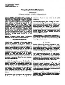
Consider the example shown in Figure 5, where 3 tasks are activated at time 3, 8 and 10 sec (Activations on the figure) with deadlines at 40, 50 and 55, respectively. There is also a pre-defined transmission slot in which the system is forced to transmit. Without such a constraint on transmission, tasks would have started as soon as they became active, running at the maximum allowed speed (dashed line). Using only DPM, task executions would be postponed as much as possible up to their deadlines, leading to the continuous line starting at t = 25, with slope equal to the maximum allowed execution speed. Notice however, that tasks could start earlier, at time t = 15, and run at a reduced speed to better exploit the transmission bandwidth (continuous line starting at t = 15sec). Such an example motivates the need for combining DVS and DPM techniques to select the most appropriate delay and speed that reduces energy consumption, while coping with the available transmission bandwidth and guaranteeing the application timing constraints. The proposed algorithm is referred to as the Energy Aware Scheduler (EAS). The EAS algorithm is applied at a generic time instant t. First, it computes the interval [tmin , tmax ] for the next activation point ta that satisfies DPM requirements and timing constraints. Second, the DPM is applied to compute the maximum tf eas at which the processor can start executing at its maximum speed smax , keeping the task set schedulable. Third, task executions are postponed as much as possible assuming execution at the maximum speed smax , to approach the starting point tBs of the transmission bandwidth. The final step is to select the minimum processor speed s needed to keep the task set schedulable. To take message communication into account, the schedule is arranged to overlap with the bandwidth allocated slot. In this way, message transmission corresponds to task execution, allowing saving more energy. The objective of the EAS algorithm is to compute the activation time ta that minimizes energy consumption in the next task schedul-

Proc. of the 10th Int. Conference on Embedded Software (EMSOFT 2010), Scottsdale, Arizona (USA), October 24-29, 2010 sbf

The system energy consumption E(ta ) is computed as E(ta ) = (ta − t)Pσ/s + (tF − ta )Pa (s(ta )fmax ) + +2Ea−σ + Eradio (t, tF ),

which is done according to the consumption models detailed in the previous section. In particular Eradio (t, tF ) is the energy the transceiver consumes in [t, tF ] as a function of the available bandwidth and Pσ/s is the not-working power consumption, which is equal to Pσ if ta − t ≥ 2ta−σ , and Ps otherwise.

EXEC

BANDWIDTH

15

25

40

50 55

time(sec)

As already said, the problem to be solved is to find ta in the interval [tmin , tmax ] that minimizes energy consumption. That is, ta | minta ∈[tmin ,tmax ] {E(ta )}.

Activations

Deadlines

ing and message transmission slot. Any valid activation point ta must take into account the feasibility bound tf eas , the start time of the bandwidth slot tBs , and the next activation time tact 1 . Such dependencies define the interval [tmin , tmax ] for ta . The value tmax is the minimum between tf eas and tBs . If the processor has no pending jobs, the value of tmin is set to the next activation time tact , otherwise tmin = t. By the definition of the interval [tmin , tmax ], the actual selection of ta is done by computing the time that minimizes the energy consumption from the current time t to the end of the evaluation period tF (discussed in Section 4). Algorithm 1 reports the sequence of steps of the EAS algorithm, while Figure 6 depicts the EAS application sequence and the result. Assumed task sets feasible under EDF, the feasibility of those task sets scheduled according the EAS is guaranteed by construction because at each step the feasibility is kept. In other words, the EAS applies the available slack to put in sleep the processor and it tries to reduce the CPU execution speed. Due to the assumptions on the system model, the bandwidth is a constraints only for the energy saving problem and it does not affect the schedulability of the task sets. Algorithm 1 Energy Aware Scheduling - EAS procedure t | t ∈ /B Compute the dbf (t); Compute sbf l∗ (t) = sbf l (t, fmax ) and obtain tf eas ; Calculate tmax = min{tf eas , tBs }; if No pending jobs at t then tmin = tact ; else tmin = t; end if Find ta ∈ [tmin , tmax ] | minta E(ta ); if ta ≥ t + 2ta−σ then Put the processor in sleep state in [t, ta ]; else Put the processor in standby in [t, ta ]; end if Compute the min frequency fa or slope sa guaranteeing feasibility. tact is the first task activation time after the actual time t.

(4)

In the next section, such a relationship will be deeply exploited by comparing the energy saving contributions from DVS and DPM.

Figure 5: An example of Energy Aware Scheduling that applies DVS and DPM and copes with the transmission bandwidth.

1

(3)

sbf

EXEC

BANDWIDTH

t

time

ta tBs tf eas ta−σ

Activations

Deadlines

Figure 6: Feasibility and bandwidth guarantee: EAS algorithm with three possible processor executions together with the time instants when are applied.

4.

ENERGY AWARE SCHEDULING: IMPLEMENTATION DETAILS

The previous section illustrated how to combine DVS and DPM techniques to save energy consumption and meet timing constraints. The constrained transmission bandwidth is assumed to be provided by the network coordinator. In this way we can concentrate on the node behavior and its energy saving strategies. In this section, we focus on some characteristics of the algorithm to better understand its behavior. We first analyze how to select the instants at which the algorithm has to be executed. Then, a more detailed analysis of the energy minimization problem is carried out. Finally, the computational cost of the method is evaluated.

4.1

EAS Applicability

The EAS algorithm has been developed to be applied at each scheduling point, such as job activation and termination, preemption points, etc. To better exploit the advantages of DPM, the algorithm should be executed when the ready queue becomes empty and the processor is going to enter the idle state. Another point where the EAS algorithm can be conveniently applied is when the bandwidth slot ends, tBe . Indeed, by forcing the processor to be active during the transmission bandwidth interval, the possibility of reclaiming some

Proc. of the 10th Int. Conference on Embedded Software (EMSOFT 2010), Scottsdale, Arizona (USA), October 24-29, 2010 slack time for the running tasks increases. Vice versa, any processor idle time inside the bandwidth slot is not an interesting point to apply the EAS algorithm, because we assumed the processor speed is selected at the beginning of the processor active period and cannot change until the end of the slot. Note that, in this work, the bandwidth is considered as a constraint, and it is assumed it is enough to transmit all the messages produced by the task set2 .

4.2

Case 2: Execution starts at the transmission bandwidth. In this case, tf eas occurs after the beginning of the transmission bandwidth, and the processor activation can be advanced at the beginning of the bandwidth tBs , as illustrated in Figure 7(b). The EAS algorithm tends to overlap the processor activation time ta to the beginning of the bandwidth to cope with the bandwidth constraint and save more energy. Note that ta can still be different than tBs , because it is the result of the energy minimization problem. If ta = tBs , the energy consumption is Pσ (ta − t) + [Pa (s(ta )) + Pon ](tBe − tBs ),

Scenarios

We have defined two scenarios to consider the typical situations that can occur during system execution. We assume that at the current time t, either the ready queue just became empty, or the transmission slot just ended. Depending on the next bandwidth chunk and on the processor demand of the task set (after t), there are different possible start times for the tasks, resulting in different energy consumptions.

which differs from the previous case by the term Pa (s(ta ))(tBs − ta ), since there is no energy consumption before the slot. Whenever ta = tBs , it is also possible to anticipate the task execution with respect to tBs to allow tasks producing messages ready to be transmitted at the beginning of the slot. In this way, the bandwidth would be better exploited by the nodes, even though the energy consumption slightly deteriorates.

4.3

EXEC

EXEC BANDWIDTH

ta Activations

Deadlines

(a) Case 1: the feasibility analysis forces the execution to start before the bandwidth

Energy Minimization

The EAS algorithm is applied to compute the next execution point ta for the processor, where ta depends on the processor speed s and on the range [tmin , tmax ]. The relationship s(ta ) among the speed and the activation point is quite intuitive and depends on the demand bound function of the task set. A heavy loaded processor results in a higher dbf and consequently in a higher speed for guaranteeing the task set. Due to such a dependency, a closed-form formula for s(ta ) cannot be derived. However, the function is convex because defined as the maximum of straight lines with slope y starting at ta , x−ta def

s(ta ) = max{

EXEC

EXEC

y } x − ta

∀x, y ∈ dbf.

Each (x, y) is a point of the dbf where the slope/speed can be controlled.

BANDWIDTH

ta Activations

Deadlines

The dependency of the execution speed sa from the task set and the associated dbf is shown in Figure 8 for a simulated case. Note the convexity of the function which depends on the utilization of the system.

(b) Case 2: execution can start at the beginning of the bandwidth Figure 7: Scenarios: the execution starts before or at the beginning of the transmission bandwidth

1

Utilization = 0.36 Utilization = 0.56

0.9

Case 1: Execution starts before the transmission bandwidth. In this case, the application is required to execute before the beginning of the bandwidth (ta ≤ tBs ), as depicted in Figure 7(a). In this case, the energy consumption is Pσ (ta − t) + Pa (s(ta ))(tBs − ta ) + [Pa (s(ta )) + +Pon ](tBe − tBs ) which is given by the cost of the processor for executing before the bandwidth (Pa (s(ta ))(tBs − ta )), the cost of the mandatory execution and transmission inside the bandwidth, and the transceiver energy cost due to the transmission bandwidth ([Pa (s(ta )) + Pon ](tBe − tBs )). 2 In the future, we plan to consider the bandwidth as a resource to be optimized, together with the system energy.

Slope

0.8 0.7 0.6 0.5 0.4 200

202

204

206

208

210

Time [ms]

Figure 8: Slope/activation time relationship s(ta ) depending on the demand bound function. Two task set with utilization U = 0.36 and U = 0.56 respectively. The energy consumption E(ta ), computed by Equation 4, has to be minimized by evaluating the energy and workload requirements in [t, tF ]. The end instant tF depends on the next time at which the EAS algorithm will be executed, which could be either the next scheduling idle time or the end of the bandwidth slot tBe . Such a

Proc. of the 10th Int. Conference on Embedded Software (EMSOFT 2010), Scottsdale, Arizona (USA), October 24-29, 2010 2. The computation of tf eas requires to compute the intersection of sbf l∗ with the x-axes, which takes O(m), where m is the number of deadlines until the next idle time.

dependency is a consequence of the policy applied, which generates different services and workload. In particular, pure DVS advancing execution at the beginning of the interval could provide different computational resources than combining DVS and DPM, which would postpone the execution at ta , with ta ≥ t. Figure 9 illustrates the different services provided in the same interval by varying the execution speed and the processor activation point ta . To resolve the previous dependency we decouple the ending instant tF from ta by choosing tF as the maximum among the scheduling idle times. The DVS applied at the beginning of the interval (time t) with the minimum feasible speed results in maximizing the time distance between t and the beginning of the next idle time, keeping the time constraints guarantee. The value of tF is the minimum between the DVS idle time and the tbE . For computing the activation time ta that minimizes the energy consumption E(ta ) we must take into account the service supplied by the processor during the interval [ta , tF ]. In particular, the function to be minimized is not the plain energy, but the ratio between the energy required in the interval [t, tF ], with the chosen ta , and the service supplied in that interval S(ta ) = (tF − ta )sa . Hence, ta | min ta

E(ta ) . S(ta )

(5)

sbf (t, s)

3. The computation of the two bounds tmin and tmax has a complexity of O(n), due to the min/max operations and the search for tact . 4. Finally, finding ta means finding ta | min E(ta ). To solve this we have applied the bisection method which has a polynomial complexity. Taking into account all the contributions, the EAS has a polynomial complexity, which makes it applicable on-line.

5.

SIMULATIONS

This section presents some simulation results achieved on the proposed EAS method. An event-driven scheduler and an energy controller simulator has been implemented in C language and interfaced to Gnuplot.

5.1

Simulation Setup

The simulator receives a task set and a bandwidth assignment as inputs. The task set is executed with a chosen scheduling policy. The energy consumed to schedule tasks and to transmit messages is computed at each simulation run. A simulation run consists of scheduling one task set with the assigned bandwidth until the task E in the hyperpeset hyperperiod hyp. The power consumption hyp riod is then considered. The scheduling policies applied are:

δ

time

Figure 9: Different services sbf provided in an interval δ by different execution policy applied. The EAS algorithm looks for the minimum ratio E(ta )/S(ta ) by spanning s(ta ) and varying ta . From equations 3 and 5, E(ta ) results to be convex in the interval [tmin , tmax ]. The convexity is guaranteed because Equation 3 is the composition of linear functions (Pσ (ta − t)), convex functions (Pa (s(ta ))) and convex functions multiplied by linear and positive functions in such an interval a) is convex, as well as the ratio (Pa (s(ta ))(t − tF ). The ratio E(t S(ta ) between a convex function and a linear function. Given the convexa) ity of E(t , the minimum exists and can be found with well known S(ta ) and efficient methods. The bisection method was used in this work. Notice that the case ta = tmin represents the condition in which the DVS effect is prominent with respect to the DPM one. Vice versa, ta = tmax represents the case in which DPM dominates over DVS.

4.4

Computational Cost

The complexity of the EAS algorithm comes form the components of the algorithm itself. In particular: 1. The computation of the dbf has a polynomial complexity O(n), where n is the number of tasks activations in the analysis interval [t, tF ];

• EDF with no energy considerations, meaning that the processor is assumed always active at the maximum frequency, even if tasks are not ready to execute. • pureDVS on top of an EDF scheduling algorithm. Only speed scaling is applied off-line to guarantee feasibility and the processor speed is set to that value. Online changes are not allowed. • pureDPM where the task execution is postponed as much as possible and then scheduled by EDF. The execution is at the maximum processor speed. • DVS and DPM are combined with EDF through the EAS algorithm. A simulator infrastructure automatically generates a stream of tuples (U, nt , B, nB ), where U denotes the utilization of the generic task set Γ, nt the number of tasks, B the communication bandwidth (expressed as a percentage of the hyperperiod), and nB the number of slots in which the bandwidth has been split. Both the task set utilization and the number of tasks are controlled by the task set assignment (U, nt ). The bandwidth assignment (B, nB ) allows to control both the total bandwidth and its distribution within the hyperperiod. Given the total utilization factor U , individual task utilizations are generated according to a uniform distribution [5]. Each bandwidth slot is set in the hyperperiod with a randomly generated offset. To reduce the bias effect of both random generation procedures, 1000

Proc. of the 10th Int. Conference on Embedded Software (EMSOFT 2010), Scottsdale, Arizona (USA), October 24-29, 2010 Average Power Consumption [Watt]

different experiments are performed for each tuples (U, nt , B, nB ) and the average is computed among the results obtained at each run.

IC

Power consumption [mW]

TI

190

SP

200

Figure 11: CPU comparison by varying the utilization; nt = 4, B = 0.3 and nB = 3. We also investigated the effects of the transmission bandwidth to the energy consumption of the system. The results are reported in Figure 12, which illustrates the power consumption as a function of the bandwidth assignment. Note how the dependency is stronger with respect to the bandwidth amount, because the transmission cost increases when there is more bandwidth available; in fact, we assumed the CPU remains active while the bandwidth is available. Moreover we assumed to have messages available to be transmitted, so that the bandwidth is fully used for transmission with an increasing cost when the assigned bandwidth increases. On the other hand, the dependency with respect to the bandwidth allocation slots (how much B is split) is quite weak. This is because message deadlines were assumed to be large enough not to create a scheduling constraint. Average Power Consumption [Watt]

TI DSPIC

D

Simulation Results

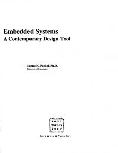
In a first simulation, we tested the power consumption of the CPUs as a function of the activation time. Figure 10 shows a general dependency of the power consumption from the model adopted for the processor. The figure shows also that both CPUs are DVS sensitive, in the sense that both privilege DVS solutions than the pure DPM ones. Indeed, the DSPIC and the TI exhibit a lower energy at tmin than at tmax (respectively 160 and 195 in this case as one of the interval of analysis along the whole execution interval). This means that a pure DVS solution costs less than a pure DPM one. Moreover, the DSPIC shows a global minimum inside the interval, meaning that a combined policy is able to reduce energy consumption. The time value corresponding to the minimum is the ta that has to be found.

IC

5.2

0 TI

Table 3: CC2420 Transceiver power profile.

0.05

SP

Pa [mWatt] 62.04

0.1

D

Ps [mWatt] 0.066

0.15

IC

Transceiver CC2420

Utilization = 0.9

0.2

SP

Table 2: Power profiles for processing devices.

Utilization = 0.6

TI

f Pa (s) Pσ tsw [fmin , fmax ] [a0 , a1 , a2 , a3 ] [mWatt] [Mhz] [mWatt] [mWatt] [sec] TI − [25, 200] [7.7489, 17.5, 168.0, 0.0] 0.12 0.00125 DSPIC 9.9 [10, 40] [25.93, 246.12, 5.6, 0.0] 1.49 0.020 Ps

CPU

Utilization = 0.3 0.25

D

Two different CPUs have been considered: the Microchip DsPic (DSPIC)3 and the Texas Instruments (TI)4 , both using the CC2420 transceiver as communication device. Table 2 and Table 3 report the parameters that characterize the power model of the processors and the transceiver used in these tests, according to the models described in Section 2. Minimum and maximum frequencies of the CPUs are taken from the device data-sheets, whereas the coefficients [a0 , a1 , a2 , a3 ] comes form Equation 1.

0.3

0.16 0.14 0.12

5

0.6

4 3 # of slots

2

1

0.3

0.4

0.7

0.8

0.5 Bandwidth

Figure 12: Average power consumption varying the bandwidth assignment; U = 0.3, nt = 4.

180 170 160 150 140 160

165

170

175

180

185

190

195

Figure 13 shows how the EAS policy is affected by the task set, in terms of U and n. Notice that the power consumption is significantly affected by the utilization but not much by the number of tasks.

Time [ms]

Figure 10: Energy consumption in one interval with the two CPUs and the same task set. The energy is obtained by varying the activation time ta within [tmin , tmax ]. Figure 11 compares the two architectures, showing a higher energy consumption for the DSPIC. The power consumption has been averaged to the hyperperiod of each task set. Note that both the CPUs have a dependency on the utilization. 3 4

DSPIC33FJ256MC710 microprocessor TMS320VC5509 Fixed-Point Digital Signal Processor

Figure 14 compares the EAS policy with respect to the pureDVS. The results are quite similar, since the considered CPUs are both sensitive to DVS. Nevertheless, the EAS is able to exploit the DPM capabilities and the available bandwidth to reduce the power consumption in all the task set assignments, mainly when the processor is not heavily loaded (low utilization cases). Finally, Figure 15 and Figure 16 compare the four scheduling policies (for TI and DSPIC, respectively), under the same B, nB , and nt conditions, but for different task set utilizations. Notice how the EAS policy outperforms the other policies, especially for low utilizations. For high utilization, EAS and pureDVS exhibit the

Proc. of the 10th Int. Conference on Embedded Software (EMSOFT 2010), Scottsdale, Arizona (USA), October 24-29, 2010 same performance (but lower power consumption with respect to the pureDPM and EDF). This happens because, for high utilization there is no room for DPM improvements and only DVS is effective. Also note that, for very low utilizations, pureDPM provides better results than pureDVS. This is due to the fact that U = 0.1 would require a speed lower than the TI minimal speed, hence pureDVS forces the CPU to have a speed greater than the utilization, providing more service than required.

Average Power Consuption [Watt]

0.2

EAS

0.15

0.1

0.1

0.2

0.3

0.4 0.5 Utilization

0.6

0.7

0.8

Figure 15: Average power consumption by varying U . All the policies are applied with B = 0.5, nB = 3 and nt = 4 and the TI processor is considered. 0.32

0.2 0.1

5

4 3 # of tasks

2

1

0.8 0.7 0.6 0.5 0.4 0.3 Utilization 0.2 0.1

Average Power Consumption [Watt]

Figure 13: Average power consumption by varying U and nt . EAS policy applied with B = 0.5 and nB = 3 and the TI processor.

DVS EAS

0.25

0.3 EDF DPM DVS EAS

0.28 0.26 0.24 0.22 0.2 0.18 0.16 0.14 0.12 0.3

0.4

0.5

0.6 Utilization

0.7

0.8

0.9

Figure 16: Average power consumption by varying U . All the policies are applied with B = 0.5, nB = 3 and nt = 4 and the DSPIC processor is considered.

0.125 0.0625

5

4 3 # of tasks

2

1

0.1

0.5 0.3 Utilization

0.7

Figure 14: Average power consumption by varying U and nt . The two policies applied with B = 0.5 and nB = 3 and the TI processor.

6.

EDF DPM DVS

0.25

0.05

Average Power Consuption [Watt]

Average Power Consumption [Watt]

To conclude, the EAS algorithm is proved to be effective with respect to the other policies because it looks for the minimum energy consumption in [tmin , tmax ] and in any possible condition. If the minimum is found in tmin or tmax , the combined method is equivalent to the pure DVS or the pure DPM, respectively. Most of the time, however, the minimum is found inside the [tmin , tmax ] interval, so that the EAS is able to further reduce energy consumption with respect to the pure versions.

0.3

CONCLUSIONS

In this paper we have presented a first stage analysis of distributed embedded systems, where nodes communicate via control or data messages. The functional aspects of a single node of a complex architecture have been investigated in order to provide real-time guarantees on applications with given timing constraints, including the provided transmission bandwidth. An on-line energy-aware scheduling algorithm (EAS) has been presented, capable of reducing the energy consumption of each node,

while guaranteeing a real-time behavior of the task set, under bandwidth constraints. A set of simulation experiments, carried out for comparing the proposed method with other scheduling approaches, showed the effectiveness of our solution under different scheduling and bandwidth conditions. As a future work, we intend to consider the bandwidth as a resource that can be optimized together with the energy, thus relaxing some of the assumptions made in this paper and making the algorithm more general.

7.

REFERENCES

[1] H. Aydin, R. Melhem, D. Mossé, and P. Mejía-Alvarez. Dynamic and aggressive scheduling techniques for power-aware real-time systems. In Proceedings of the 22nd IEEE Real-Time Systems Symposium (RTSS), pages 95–105, 2001. [2] H. Aydin, R. Melhem, D. Mossé, and P. Mejia Alvarez. Power-aware scheduling for periodic real-time tasks. IEEE Transactions on Computers, 53(5):584–600, May 2004. [3] S. K. Baruah. Dynamic- and static-priority scheduling of

Proc. of the 10th Int. Conference on Embedded Software (EMSOFT 2010), Scottsdale, Arizona (USA), October 24-29, 2010

[4]

[5]

[6]

[7]

[8]

[9]

[10]

[11]

[12]

[13]

[14]

[15]

[16]

recurring real-time tasks. Real-Time Syst., 24(1):93–128, 2003. S. K. Baruah, A. K. Mok, and L. E. Rosier. Preemptively scheduling hard-real-time sporadic tasks on one processor. In In Proceedings of the 11th Real-Time Systems Symposium, pages 182–190. IEEE Computer Society Press, 1990. E. Bini and G. C. Buttazzo. Biasing effects in schedulability measures. In Proceedings of the 16th Euromicro Conference on Real-Time Systems, Catania, Italy, June 2004. J.-J. Chen and T.-W. Kuo. Procrastination determination for periodic real-time tasks in leakage-aware dynamic voltage scaling systems. In ICCAD ’07: Proceedings of the 2009 International Conference on Computer-Aided Design, pages 289–294, New York, NY, USA, 2007. ACM. J.-J. Chen and T.-W. Kuo. Procrastination determination for periodic real-time tasks in leakage-aware dynamic voltage scaling systems. In International Conference on Computer-Aided Design (ICCAD), pages 289–294, 2007. N. Christian, M. Mauro, S. Luca, P. Paolo, L. Giuseppe, and F. Gianluca. Baccarat: a dynamic real-time bandwidth allocationpolicy for ieee 802.15.4. In Proceedings of IEEE Percom 2010, International Workshop on Sensor Networks and Systems for Pervasive Computing (PerSeNS 2010), Mannheim, Germany, 2010. V. Devadas and H. Aydin. On the interpaly of dynamic volatage scaling and dynamic power management in real-time embedded applications. In EMSOFT’08: Proceedings of the 8th ACM Conference on Embedded Systems Software, pages 99–108, New York, NY, USA, 2008. ACM. K. Huang, L. Santinelli, J.-J. Chen, L. Thiele, and G. Buttazzo. Adaptive dynamic power management for hard real-time systems. In RTSS’09: Proceedings of the 30th IEEE Real-Time Systems Symposium, Washington, DC, USA, 2009. IEEE Computer Society. K. Huang, L. Santinelli, J.-J. Chen, L. Thiele, and G. Buttazzo. Periodic power management schemes for real-time event streams. In CDC’09: Proceedings of the 48th IEEE Conference on Decision and Control, pages 6224 – 6231, Washington, DC, USA, 2009. IEEE Computer Society. R. Jejurikar, C. Pereira, and R. Gupta. Leakage aware dynamic voltage scaling for real-time embedded systems. In Proceedings of the 41st ACM/IEEE Design Automation Conference (DAC), pages 275–280, 2004. N. S. Kim, T. Austin, D. Blaauw, T. Mudge, K. Flautner, J. S. Hu, M. J. Irwin, M. Kandemir, and V. Narayanan. Leakage current: Moore’s law meets static power. Computer, 36:68–75, 2003. W. Kim, D. Shin, H. Yun, J. Kim, and S. Min. Performance camparision of dynamic voltage scaling algorithms for hard real-time systems. In Proc. 8th IEEE Real-Time and Embedded Technology and Applications Symp., pages 219–228, San Jose, California, September 2002. A. Koubâa, M. Alves, E. Tovar, and A. Cunha. An implicit gts allocation mechanism in ieee 802.15.4 for time-sensitive wireless sensor networks: theory and practice. Real-Time Syst., 39(1-3):169–204, 2008. G. S. A. Kumar and G. Manimaran. Energy-aware scheduling of real-time tasks in wireless networked embedded systems. In RTSS ’07: Proceedings of the 28th IEEE International Real-Time Systems Symposium, pages

[17]

[18]

[19]

[20]

[21]

[22]

[23]

[24]

[25]

[26]

[27]

[28]

15–24, Washington, DC, USA, 2007. IEEE Computer Society. T. Martin and D. Siewiorek. Non-ideal battery and main memory effects on cpu speed-setting for low power. IEEE Transactions on VLSI Systems, 9(1):29–34, 2001. B. Mochocki, D. Rajan, X. S. Hu, C. Poellabauer, K. Otten, and T. Chantem. Network-aware dynamic voltage and frequency scaling. In RTAS ’07: Proceedings of the 13th IEEE Real Time and Embedded Technology and Applications Symposium, pages 215–224, Washington, DC, USA, 2007. IEEE Computer Society. P. Pillai and K. G. Shin. Real-time dynamic voltage scaling for low-power embedded operating systems. In SOSP ’01: Proceedings of the 18th ACM Symposium on Operating Systems Principles, pages 89–102, Washington, DC, USA, 2008. IEEE Computer Society. C. Schurgers, V. Raghunathan, and M. B. Srivastave. Modulation scaling for real-time energy aware packet scheduling. In Global Telecommunications Conferance (GLOBECOMM 01), pages 3653–3657, San Antonio, Texas (USA), 2001. K. Seth, A. Anantaraman, F. Mueller, and E. Rotenberg. Fast: Frequency-aware static timing analysis. In Proc. 24th IEEE Real-Time Systems Symposium, pages 40–51, Cancun, Mexico, December 2003. I. Shin and I. Lee. Compositional real-time scheduling framework with periodic model. ACM Trans. Embed. Comput. Syst., 7(3):1–39, 2008. C.-Y. Yang, J.-J. Chen, C.-M. Hung, and T.-W. Kuo. System-level energy-efficiency for real-time tasks. In the 10th IEEE International Symposium on Object/component/service-oriented Real-time distributed Computing (ISORC), pages 266–273, 2007. F. Yao, A. Demers, and S. Shenker. A scheduling model for reduced CPU energy. In Proceedings of the 36th Annual Symposium on Foundations of Computer Science (FOCS), pages 374–382, 1995. J. Yi, C. Poellabauer, X. S. Hu, J. Simmer, and L. Zhang. Energy-conscious co-scheduling of tasks and packets in wireless real-time environments. In RTAS ’09: Proceedings of the 2009 15th IEEE Real-Time and Embedded Technology and Applications Symposium, pages 265–274, Washington, DC, USA, 2009. IEEE Computer Society. Y. Zhang, X. Hu, and D. Z. Chen. Task scheduling and voltage selection for energy minimization. In Proceedings of the 39th ACM/IEEE Design Automation Conference (DAC), pages 183–188, 2002. B. Zhao and H. Aydin. Minimizing expected energy consumption through optimal integration of dvs and dpm. In ICCAD ’09: Proceedings of the 2009 International Conference on Computer-Aided Design, pages 449–456, New York, NY, USA, 2009. ACM. J. Zhuo and C. Chakrabarti. System-level energy-efficient dynamic task scheduling. In Proceedings of the 42nd ACM/IEEE Design Automation Conference(DAC), pages 628–631, 2005.