Requirements Validation for Hybrid Systems - Embedded Systems

Requirements Validation for Hybrid Systems? Alessandro Cimatti, Marco Roveri, and Stefano Tonetta Fondazione Bruno Kessler (FBK-irst), Trento, Italy

Abstract. The importance of requirements for the whole development flow calls for strong validation techniques based on formal methods. In the case of discrete systems, some approaches based on temporal logic satisfiability are gaining increasing momentum. However, in many real-world domains (e.g. railways signaling), the requirements constrain the temporal evolution of both discrete and continuous variables. These hybrid domains pose substantial problems: on one side, a continuous domain requires very expressive formal languages; on the other side, the resulting expressiveness results in highly intractable problems. In this paper, we address the problem of requirements validation for real-world hybrid domains, and present two main contributions. First, we propose the HRELTL logic, that extends the Linear-time Temporal Logic with Regular Expressions (RELTL) with hybrid aspects. Second, we show that the satisfiability problem for the linear fragment can be reduced to an equi-satisfiable problem for RELTL. This makes it possible to use automatic (albeit incomplete) techniques based on Bounded Model Checking and on Satisfiability Modulo Theory. The choice of the language is inspired by and validated within a project funded by the European Railway Agency, on the formalization and validation of the European Train Control System specifications. The activity showed that most of requirements can be formalized into HRELTL, and an experimental evaluation confirmed the practicality of the analyses.

1

Introduction

Requirements analysis is a fundamental step in the development process of software and system design. In fact, flaws and ambiguities in the requirements can lead to the development of correct systems that do not do what they were supposed to. This is often unacceptable, especially in safety-critical domains, and calls for strong tools for requirements validation based on formal techniques. The problem of requirements validation is significantly different from traditional formal verification, where a system model (the entity under analysis) is compared against a set of requirements (formalized as properties in a temporal logic), which are assumed to be “golden”. In requirements validation, on the contrary, there is no system to be analyzed (yet), and the requirements themselves are the entity under analysis. Formal methods for requirements validation are being devoted increasing interest [12, 15, 27, 1]. In such approaches, referred to as property-based, the requirements are represented as statements in some temporal logics. This allows to retain a correspondence between the informal requirements and the formal statement, and gives the ?

The first and second authors are supported by the European Commission (FP7-2007-IST-1217069 COCONUT). The third author is supported by the Provincia Autonoma di Trento (project ANACONDA).

ability to reason at the level of abstraction of the requirements engineer. Typical analysis functionalities include the ability to check whether the specification is consistent, whether it is strict enough to rule out some undesirable behaviors, and whether it is weak enough not to rule out some desirable scenarios. These analysis functionalities can in turn be obtained by reduction to temporal logics satisfiability [27]. Property-based approaches have been typically applied in digital domains, where the requirements are intended to specify a set of behaviors over discrete variables, and the wealth of results and tools in temporal logic and model checking provides a substantial technological basis. However, in many real-world domains (e.g. railways, space, industrial control), the requirements are intended to constrain the evolution over time of a combination of discrete and continuous variables. Hybrid domains pose substantial problems: on the one side, a continuous domain requires very expressive formal languages; on the other side, the high expressiveness leads to highly intractable problems. In this paper, we address the problem of requirements validation in such hybrid domains by making two main contributions. First, we define a suitable logic for the representation of requirements in hybrid domains. The logic, called Hybrid Linear Temporal Logic with Regular Expressions (HRELTL), is interpreted over hybrid traces. This allows to evaluate constraints on continuous evolutions as well as discrete changes. The basic atoms (predicates) of the logic include continuous variables and their derivatives over time, and are interpreted both over time points and over open time intervals.1 The semantics relies on the fact that each open interval of a hybrid trace can be split if it does not have a uniform evaluation of predicates in the temporal formulas under analysis (cf. [26, 13]), and that the formulas satisfy properties of sample invariance and finite variability [13]. The logic encompasses regular expressions and linear-time operators, and suitable choices have been made to interpret the “next” operator and regular expressions over the open time intervals, and the derivative of continuous variables over the time points. Second, we define a translation method for automated verification. The translation encodes satisfiability problems for the linear fragment of HRELTL into an equisatisfiable problem in a logic over discrete traces. The restrictions of the linear fragment guarantee that if the formula is satisfiable, there exists a piecewise-linear solution. We exploit the linearity of the predicates with regard to the continuous variables to encode the continuity of the function into quantifier-free constraints. We can therefore compile the resulting formula into a fair transition system and use it to solve the satisfiability and the model checking problem with an automata-theoretic approach. We apply infinitestate model checking techniques to verify the language emptiness of the resulting fair transition system. Our work has been inspired by and applied within a project funded by the European Railway Agency (http://www.era.europa.eu). The aim of the project was to develop a methodology supported by a tool for the validation of requirements in railway domains. Within the project, we collaborated with domain experts in a team that tackled the formalization of substantial fragments of the European Train Control System (ETCS) specification. With regard to the hybrid aspects of ETCS requirements, the formaliza1

This is known to be a nontrivial issue: see for instance [26, 13, 22] for a discussion on which type of intervals and hybrid traces must be considered.

2

LRBG Section Time−out stop location

Distance to Danger Point Length of overlap Section Time−out stop location Overlap Time−out start location

Optional signal End Section Time−out start location Section(1)

Section(2) = End Section

Fig. 1. Structure of an MA (left) and a speed monitoring curve (right) [14].

tion and the validation were based on the language and techniques described in this paper, and were successfully applied by the domain experts.

2

Motivating Application Domain

The ETCS specification is a set of requirements related to the automatic supervision of the location and speed performed by the train on-board system. The system is intended to be progressively installed on all European trains in order to guarantee the interoperability with the track-side system which are currently governed by national rules. ETCS specifies how the train should behave in the proximity of the target location. In particular, the Chapter 3 of the System Requirement Specification (SRS) [14] describes how trains move on a line and periodically receive a so-called Movement Authority (MA). The MA consists of a set of sections and a series of timeout that define some deadlines of the authorization to move in each section while a number of curves limit the speed of the train approaching the end of the MA (see Fig. 1). The specific curves are not defined by ETCS, but only constrained by high-level requirements (“The algorithm for their calculation is an implementation matter” SRS Sec. 3.13.4.1). Moreover, when the trains pass some limit, particular actions must be taken on board: e.g. when the train passes the end of the MA the “train trip” must be started. The ETCS specification poses demanding requisites to the formal methods adopted for its validation. First, the adopted formalism shall be able to capture the meaning of the requirements. Second, the formalism shall be as simple as possible to be used by non-experts in formal methods: the requirements are usually ambiguous English sentences that only an expert in the domain can formalize and validate. In this context, a model-based approach is not natural. First, designing a hybrid system that captures all behaviors allowed by the requirements requires to consider all possible intricate combinations of timeout values, locations where to reset the timers, speed limits for given locations. Second, these are not parameters of the system but variables that change their value at discrete steps. Finally, in a model-based approach it is hard to maintain the link between a requirement and its formal counterpart in the model. A property-based approach to requirements validation relies on the availability of an expressive temporal logic, so that each informal statement has a formal counterpart with similar structure. A natural choice are formulas in Linear-time Temporal Logic (LTL) [25] extended with Regular Expressions (RELTL) [6], because temporal formulas often resemble their informal counterpart. This is of paramount importance when 3

experts in the application domain have the task of disambiguating and formalizing the requirements. For instance, a complex statement such as “The train trip shall issue an emergency brake command, which shall not be revoked until the train has reached standstill and the driver has acknowledged the trip” SRS Sec. 3.13.8.2 can be formalized into G (train trip → (emergency brake U (train speed = 0 ∧ ack trip))). In order to deal with an application domain such as ETCS, first, we need to model the dynamic of continuous variables, such as position, speed, time elapse, and timers, in a way that is reasonably accurate from the physical point of view. For example, we expect that a train can not move forward and reach a location without passing over all intermediate positions. Second, we must be able to express properties of continuous variables over time intervals. This poses problems of the satisfiability of formulas like (pos ≤ P U pos > P ) or (speed > 0 U speed = 0). The first formula is satisfiable only if we consider left-open intervals, while the second one is satisfiable only if we consider left-closed intervals (see [22]). Considering time points (closed singular intervals) and open intervals is enough fine grained to represent all kinds of intervals. Last, we need to be able to intermix continuous evolution and discrete steps, intuitively modeling “instantaneous” changes in the status of modes and control procedures. For example, the requirement “The End Section timer shall be started on-board when the train passes the End Section timer start location” (SRS Sec. 3.8.4.1.1) demands to interrupt the continuous progress of the train for resetting a timer.

3

Hybrid traces

Let V be the finite disjoint union of the sets of variables VD (with a discrete evolution) and VC (with a continuous evolution) with values over the Reals.2 A state s is an assignment to the variables of V (s : V → R). We write Σ for the set of states. Let f : R → Σ be a function describing a continuous evolution. We define the projection of f over a variable v, written f v , as f v (t) = ˙ f (t)(v). We say that a function f : R → R is piecewise analytic iff there exists a sequence of adjacent intervals J0 , J1 , ... ⊆ R and a sequence of analytic functions h0 , h1 , ... such that ∪i Ji = R, and for all i ∈ N, f (t) = hi (t) for all t ∈ Ji . Note that, if f is piecewise analytic, the left and right derivatives exist in all points. We denote with f˙ the derivative of a real function f , with f˙(t)− and f˙(t)+ the left and the right derivatives respectively of f in t. Let I be an interval of R or N; we denote with le(I) and ue(I) the lower and upper endpoints of I, respectively. We denote with R+ the set of non-negative real numbers. Hybrid traces describe the evolution of variables in every point of time. Such evolution is allowed to have a countable number of discontinuous points corresponding to changes in the discrete part of the model. These points are usually called discrete steps, while we refer to the period of time between two discrete steps as continuous evolution. Definition 1 (Hybrid Trace). A hybrid trace over V is a sequence ˙ hf0 , I0 i, hf1 , I1 i, hf2 , I2 i, . . . such that, for all i ∈ N, hf , Ii = – either Ii is an open interval (Ii = (t, t0 ) for some t, t0 ∈ R+ , t < t0 ) or is a singular interval (Ii = [t, t] for some t ∈ R+ ); 2

In practice, we consider also Boolean and Integer variables with a discrete evolution, but we ignore them to simplify the presentation.

4

– the intervals are adjacent, S i.e. ue(Ii ) = le(Ii+1 ); – the intervals cover R+ : i∈N Ii = R+ (thus I0 = [0, 0]); – fi : R → Σ is a function such that, for all v ∈ VC , fiv is continuous and piecewise analytic, and for all v ∈ VD , fiv is constant; – if Ii = (t, t0 ) then fi (t) = fi−1 (t), fi (t0 ) = fi+1 (t0 ). Typically, the fi are required to be smooth. Since observable events may occur during a continuous evolution, we wish that a predicate over the continuous variable changes its truth value only a finite number of times in a bounded interval. For this reason, we require the analyticity of functions (see similar assumptions in [13]). At the same time, we weaken the condition of smoothness allowing discontinuity in the derivatives also during a continuous evolution. This allows to observe the value of functions and their derivatives without the need to break the continuous evolution with discrete steps not required by the specification. Fig. 2 shows the evolution of two continuous variables (speed and limit) and a discrete variable (warning). The evolution presents two discrete steps and three continuous evolutions. The figure shows two possible traces, respectively with 10 and 14 intervals. In the second continuous evolution the function associated to speed is continuous but not derivable in all points. Some predicate over the variables in V may evaluate to true only in particular points of a continuous evolution. Therefore, it is important to sample the evolution in particular time points. We say that a trace is a sampling refinement of another one if it has been obtained by splitting an open interval into two parts by adding a sampling point in the middle [13]. In Fig. 2, TRACE2 refines TRACE1 by exposing two more points. Definition 2 (Partitioning Function [13]). A partitioning function µ is a sequence µ0 , µ1 ,S µ2 , . . . of non-empty, adjacent and disjoint intervals of N partitioning N. Formally, i∈N µi = N and ue(µi ) = le(µi+1 ) − 1. 0

0

VALUE

Definition 3 (Trace Sampling Refinement [13]). A hybrid trace hf , I i is a sampling 0 0 refinement ofShf , Ii by the partitioning µ (denoted with hf , I i µ hf , Ii) iff, for all i ∈ N, Ii = j∈µi Ij0 and, for all j ∈ µj , fj0 = fi . speed limit warning

TIME TRACE1 TRACE2

Fig. 2. Possible evolution of two continuous variables (speed and limit) and a discrete variable (warning), and two possible hybrid traces that represent it. TRACE2 is a refinement of TRACE1.

4

A temporal logic for hybrid traces

In this section we define HRELTL, i.e. linear temporal logic extended with regular expressions equipped to deal with hybrid traces. The language is presented in a general 5

form with real arithmetic predicates without details on the syntax and the semantics of the real functions. It is indeed possible that some requirements need such expressiveness to be faithfully represented. A linear sub-case is then presented for which we have a discretization that produces equi-satisfiable formulas. Syntax. If v is a variable we denote with NEXT(v) the value of v after a discrete step and with DER(v) the derivative of v. If V is the set of variables, we denote with Vnext the set of next variables and with Vder the set of derivatives. HRELTL is built over a set of basic atoms, that are real arithmetic predicates over V ∪ Vnext , or over V ∪ Vder .3 We denote with P RED the set of predicates, with p a generic predicate, with pcurr a predicate over V only, with pnext a predicate over V and Vnext , and with pder a predicate over V and Vder . We denote with p the predicate obtained from p by replacing < with ≥, > with ≤, = with 6= and vice versa. We denote with p./ the predicate obtained from p by substituting the top-level operator with ./, for ./∈ {, =, ≤, ≥, 6=}. The subset P REDla of P RED over linear arithmetic constraints consists of the predicates in one of the following forms – a0 + a1 v1 + a2 v2 + · · · + an vn ./ 0 where v1 , . . . , vn ∈ VC , a0 , . . . , an are arithmetic predicates over variables in VD , and ./∈ {, =, ≤, ≥, 6=}. – a0 + a1 v˙ ./ 0 where v ∈ VC , a0 , a1 are arithmetic predicates over variables in VD , and ./∈ {, =, ≤, ≥, 6=}. Example 1. x ≤ y + z, NEXT(x) = 0, DER(x) ≤ d are in P RED. The first two predicates are also in P REDla , while the third one is in P REDla only if d is a discrete variable. We remark that, the class of predicates generalizes the class of constraints used for linear hybrid automata [2, 19]; in particular, we replace constants with discrete (densedomain) variables. The HRELTL is defined by combining extended regular expressions (SEREs) and temporal operators from LTL. The linear fragment of HRELTL is defined by considering only predicates in P REDla . Definition 4 (SERE syntax). If p ∈ P RED, r, r1 and r2 are SEREs, then: – p is a SERE; –  is a SERE; – r[*], r1 ; r2 , r1 : r2 , r1 | r2 , and r1 && r2 are SEREs. Definition 5 (HRELTL syntax). If p ∈ P RED, φ, φ1 and φ2 are HRELTL formulas, and r is a SERE, then: – p is a HRELTL formula; – ¬φ1 , φ1 ∧ φ2 , X φ1 , φ1 U φ2 are HRELTL formulas; – r ♦→ φ is an HRELTL formula. We use standard abbreviations for ∨, →, G , F , and |→ (see, e.g., [11]). Example 2. G (warning = 1 → (warning = 1 U speed ≤ limit)) is in HRELTL. 3

In practice, we consider also predicates with next variables and derivatives, and derivatives after a discrete step, but we ignore this extensions to simplify the presentation.

6

Semantics. Some choices underlie the definition of the semantics in order to guarantee that the satisfaction of a formula by a hybrid trace does not depend on the sampling of continuous evolutions, rather it depends only on the discrete steps and on the shape of the functions that describe the continuous evolutions (sampling invariance [13]). Other choices have been taken to make the formalization of requirements more natural. For example, predicates including next variables can be true only in discrete steps. Definition 6 (PRED semantics). – hf , Ii, i |= pcurr iff, for all t ∈ Ii , pcurr evaluates to true when v is equal to fiv (t), denoted with fi (t) |= p; – hf , Ii, i |= pnext iff there is a discrete step between i and i + 1, i.e. Ii = Ii+1 = v [t, t], and pnext evaluates to true when v is equal to fiv (t) and NEXT(v) to fi+1 (t), denoted with fi (t), fi+1 (t) |= pnext ; – hf , Ii, i |= pder iff, for all t ∈ Ii , pder evaluates to true both when v is equal to fiv (t) and DER(v) to f˙iv (t)+ , and when v is equal to fiv (t) and DER(v) to f˙iv (t)− , denoted with fi (t), f˙i (t)+ |= pder and fi (t), f˙i (t)− |= pder (when f˙i (t) is defined this means that fi (t), f˙i (t) |= pder ). Note that, for all i ∈ N, fi is defined on all reals, and thus the left and right derivatives are defined in all points of Ii . In order to ensure sample invariance, the predicates inside a SERE can be true over a sequence of more than one moment. This is different from the standard discrete approach, where they are usually true only if evaluated on just one state. Moreover, we require that if a sequence satisfies the concatenation or repetition of two SEREs, the sequence must contain a discrete step. Definition 7 (SERE semantics). – hf , Ii, i, j |= p iff, for all k, i ≤ k < j, there is no discrete step at k (Ik 6= Ik+1 ), and, for all k, i ≤ k ≤ j, hf , Ii, k |= p; – hf , Ii, i, j |=  iff i > j; – hf , Ii, i, j |= r[*] iff i > j, or hf , Ii, i, j |= r, or there exists a discrete step at k (Ik = Ik+1 ), i ≤ k < j, such that hf , Ii, i, k |= r, hf , Ii, k + 1, j |= r[*]; – hf , Ii, i, j |= r1 ; r2 iff hf , Ii, i, j |= r1 , hf , Ii, j + 1, j |= r2 (i.e., r2 accepts the empty word), or; hf , Ii, i, i − 1 |= r1 , hf , Ii, i, j |= r2 (i.e., r1 accepts the empty word), or there exists a discrete step at k (Ik = Ik+1 ), i ≤ k < j, such that hf , Ii, i, k |= r1 , hf , Ii, k + 1, j |= r2 ; – hf , Ii, i, j |= r1 : r2 iff there exists a discrete step at k (Ik = Ik+1 ), i ≤ k ≤ j, such that hf , Ii, i, k |= r1 , hf , Ii, k, j |= r2 ; – hf , Ii, i, j |= r1 | r2 iff hf , Ii, i, j |= r1 or hf , Ii, i, j |= r2 ; – hf , Ii, i, j |= r1 && r2 iff hf , Ii, i, j |= r1 and hf , Ii, i, j |= r2 . Definition 8 (HRELTL semantics). – hf , Ii, i |= p iff hf , Ii, i |= p; – hf , Ii, i |= ¬φ iff hf , Ii, i 6|= φ; – hf , Ii, i |= φ ∧ ψ iff hf , Ii, i |= φ and hf , Ii, i |= ψ; – hf , Ii, i |= X φ iff there is a discrete step at i (Ii = Ii+1 ), and hf , Ii, i + 1 |= φ; 7

– hf , Ii, i |= φ U ψ iff, for some j ≥ i, hf , Ii, j |= ψ and, for all i ≤ k < j, hf , Ii, k |= φ; – hf , Ii, i |= r ♦→ φ iff, there exists a discrete step at j ≥ i (Ij = Ij+1 ) such that hf , Ii, i, j |= r, and hf , Ii, j |= φ. Definition 9 (Ground Hybrid Trace [13]). A hybrid trace hf , Ii is a ground hybrid trace for a predicate p iff the interpretation of p is constant throughout every open interval: if Ii = (t, t0 ) then either hf , Ii, i |= p or hf , Ii, i |= p. A hybrid trace hf , Ii is a ground hybrid trace for a formula φ iff it is ground for all predicates of φ. Given an HRELTL formula φ, and a hybrid trace hf , Ii ground for φ, we say that hf , Ii |= φ iff hf , Ii, 0 |= φ. Given an HRELTL formula φ, and any hybrid trace hf , Ii, we say that hf , Ii |= φ 0 0 0 0 iff there exists a sampling refinement hf , I i of hf , Ii such that hf , I i is ground for φ 0 0 and hf , I i |= φ. For example, the hybrid traces depicted in Fig. 2 satisfy the formula of Example 2. The following theorems guarantee that the semantics is well defined. (We refer the reader to Sec. B of the appendix for the proofs.) Theorem 1 (Finite variability). Given a formula φ, for every hybrid trace hf , Ii there 0 0 exists another hybrid trace hf , I i which is a sampling refinement of hf , Ii and ground for φ. 0

0

Theorem 2 (Sample invariance). If hf , I i is a sampling refinement of hf , Ii, then the two hybrid traces satisfy the same formulas. Note that we can encode the reachability problem for linear hybrid automata into the satisfiability problem of a linear HRELTL formula. Despite the undecidability of the satisfiability problem, we provide automatic techniques to look for satisfying hybrid traces, by constructing an equi-satisfiable discrete problem.

5

Reduction to discrete semantics

RELTL is the temporal logic that combines LTL with regular expressions and constitutes the core of many specification languages. Here, we refer to a first-order version of RELTL with real arithmetic predicates. RELTL syntax can be seen as a subset of HRELTL where predicates are allowed to include only current and next variables, but not derivatives. RELTL formulas are interpreted over discrete traces. A discrete trace is a sequence of states σ = s0 , s1 , s2 , . . . with si ∈ Σ for all i ∈ N. The semantics for RELTL is analogue to the one of HRELTL but restricted to discrete steps only. We refer the reader to Sec. C for more details. Encoding Hybrid RELTL into Discrete RELTL. We now present a translation of formulas of the linear fragment of HRELTL into equi-satisfiable formulas of RELTL. In the rest of this document we assume that formulas contain only predicates in P REDla . 8

We introduce two Real variables δt and ζ respectively to track the time elapsing between two consecutive steps, and to enforce the non-Zeno property (i.e. to guarantee that time diverges). We introduce a Boolean variable ι that tracks if the current state samples a singular interval or an open interval. We define a formula ψι that encodes the possible evolution of δt and ι: ψι := ι ∧ ζ > 0 ∧ G ((ι ∧ δt = 0 ∧ X (ι)) ∨ (ι ∧ δt > 0 ∧ X (¬ι)) ∨ (¬ι ∧ δt > 0 ∧ X (ι))) ∧ G (NEXT(ζ) = ζ) ∧ G F δt ≥ ζ.

(1)

In particular, we force to have a discrete step, which is characterized by two consecutive singular intervals, if and only if δt = 0. For every continuous variable v ∈ VC we introduce the Real variable v˙ l and v˙ r that track the left and right derivative of v. We define a formula ψDER that encodes the relation among continuous variables and their derivatives: ψDER :=

V

v∈VC

((δt > 0 ∧ ι) → (NEXT(v) − v) = (δt × NEXT(v˙ l ))) ∧ ((δt > 0 ∧ ¬ι) → (NEXT(v) − v) = (δt × v˙ r )).

(2)

The equation says that, before a point that samples an open interval, the evolution is tracked with the value of left derivative assigned in the sampling point, while afterwards, the evolution is tracked with the right derivative in the same point. We define a formula ψP REDφ , being P REDφ the set of predicates occurring in φ without next variables and derivatives, that encodes the continuous evolution of the predicates. V ψP REDφ := (δt > 0 ∧ ι) → Vp∈P REDφ NEXT(p= ) → p= ∧ (δt > 0 ∧ ¬ι) → Vp∈P REDφ p= → NEXT(p= ) ∧ δt > 0 → p∈P REDφ ((p< → ¬X p> ) ∧ (p> → ¬X p< )).

(3)

The first two conjuncts encode that if p= holds in an open interval, then p= holds in the immediately adjacent singular intervals too. The third conjuncts encodes that if p< holds we cannot move to an immediately following state where p> holds (and vice versa) without passing through a state where p= holds. We define ψVD to encode that discrete variables do not change value during a continuous evolution: V ψVD := δt > 0 → (

v∈Vd ( NEXT (v)

= v)).

(4)

Finally, we define the partial translation τ 0 (φ) recursively over φ. The translation τa0 of predicates is defined as: – τa0 (pcurr ) = pcurr ; – τa0 (pnext ) = (δt = 0) ∧ pnext ; – τa0 (pder ) = pder [v˙ l /DER(v)] ∧ pder [v˙ r /DER(v)]). Where, p[v 0 /v] is predicate p where every occurrence of v is replaced with v 0 . The translation τr0 of SEREs is defined as: – τr0 (p) = (δt > 0 ∧ τa0 (p))[*] ; τa0 (p); 4 – τr0 () = ; – τr0 (r[*]) =  | {τr0 (r) : δt = 0}[*] ; τr0 (r); – τr0 (r1 ; r2 ) = {{ && τr0 (r1 )} ; τr0 (r2 )} | {τr0 (r1 ) ; { && τr0 (r2 )}} | {{τr0 (r1 ) : δt = 0} ; {τr0 (r2 ) : >}}; 4

This has the effect that τr0 (pnext ) = τa0 (pnext ) = (δt = 0 ∧ pnext ).

9

– τr0 (r1 : r2 ) = τr0 (r1 ) : δt = 0 : τr0 (r2 ); – τr0 (r1 | r2 ) = τr0 (r1 ) | τr0 (r2 ); – τr0 (r1 && r2 ) = τr0 (r1 ) && τr0 (r2 ). The translation τ 0 of HRELTL is defined as: – τ 0 (p) = τa0 (p); – τ 0 (¬φ1 ) = ¬τ 0 (φ1 ); – τ 0 (φ1 ∧ φ2 ) = τ 0 (φ1 ) ∧ τ 0 (φ2 ); – τ 0 (X φ1 ) = δt = 0 ∧ X τ 0 (φ1 ); – τ 0 (φ1 U φ2 ) = τ 0 (φ1 ) U τ 0 (φ2 ); – τ 0 (r ♦→ φ) = {τr0 (r) : δt = 0} ♦→ τ 0 (φ). Thus, the translation τ for a generic HRELTL formula is defined as: τ (φ) := ψι ∧ ψDER ∧ ψP REDφ ∧ ψVD ∧ τ 0 (φ).

(5)

Remark 1. If φ contains only quantifier-free predicates then also τ (φ) is quantifier-free. In general, the predicates in τ (φ) are non linear. φ may contain non linear predicates, even in the case φ is in the linear fragment of HRELTL, since it may contain polynomials over discrete variables or multiplications of a continuous variable with discrete variables. Moreover, Equation 2 introduces quadratic equations. Finally, note that if φ does not contain SEREs, then the translation is linear in the size of φ. We now define a mapping from the hybrid traces of φ to the discrete traces of τ (φ), and vice versa. Without loss of generality, we assume that the hybrid trace does not have discontinuous points in the derivatives in the open intervals. Definition 10. Given a hybrid trace hf , Ii, the discrete trace σ = Ω(hf , Ii) is defined as follows: for all i ∈ N, – ti = t if if Ii = [t, t], and ti = (t + t0 )/2 if Ii = (t, t0 ); – si (v) = fiv (ti ); – if Ii = (t, t0 ), si (v˙ l ) = (fiv (ti ) − fiv (ti−1 ))/(ti − ti−1 ) and si (v˙ r ) = (fiv (ti+1 ) − fiv (ti ))/(ti+1 − ti ); if Ii = [t, t] then si (v˙ l ) = f˙iv (t)− and si (v˙ r ) = f˙iv (t)+ ; – si (ι) = > if Ii = [t, t], and si (ι) = ⊥ if Ii = (t, t0 ); – si (δt ) = ti+1 − ti ; – si (ζ) = α, such that for all i ∈ N, there exists j ≥ i such that ti+1 − ti ≥ α (such α exists for the Cauchy’s condition on the divergent sequence {ti }i∈N ). We then define the mapping in the opposite direction. Definition 11. Given a discrete trace σ, the hybrid trace hf , Ii = Υ (σ) is defined as follows: for P all i ∈ N, – ti = 0≤j then Ii = [ti , ti ] else Ii = (ti−1 , ti+1 ), – if si (δt ) > 0 then fi is the piecewise linear function defined as fiv (t) = si (v) − si (v˙ l ) × (ti − t) if t ≤ ti and as fiv (t) = si (v) + si (v˙ r ) × (t − ti ) if t > ti . Theorem 3 (Equi-satisfiability). If hf , Ii is ground for φ and hf , Ii |= φ, then Ω(hf , Ii) |= τ (φ). If σ is a discrete trace such that σ |= τ (φ), then Υ (σ) |= φ and Υ (σ) is ground for φ. Thus φ and τ (φ) are equi-satisfiable. For the proofs we refer the reader to Sec. C of the appendix. 10

6

Fair transition systems and language emptiness

Fair Transition Systems (FTS) [25] are a symbolic representation of infinite-state systems. First-order formulas are used to represent the initial set of states I, the transition relation T , and each fairness condition ψ ∈ F . To check the satisfiability of an RELTL formula φ with first-order constraints we build a fair transition system Sφ and we check whether the language accepted by Sφ is not empty with standard techniques. For the compilation of the RELTL formula Sφ into an equivalent FTS Sφ we rely on the works described in [11, 10]. The language non-emptiness check for the FTS Sφ is performed by looking for a lasso-shape trace of length up to a given bound. We encode this trace into an SMT formula using a standard Bounded Model Checking (BMC) encoding and we submit it to a suitable SMT solver. This procedure is incomplete from two point of views: first, we are performing BMC limiting the number of different transitions in the trace; second, unlike the Boolean case, we cannot guarantee that if there is no lasso-shape trace, there does not exist an infinite trace satisfying the model (since a real variable may be forced to increase forever). Nevertheless, we find the procedure extremely efficient in the framework of requirements validation. The BMC encoding allows us to perform some optimizations. First, as we are considering a lasso-shape path, the Cauchy condition for the non-Zeno property can be reduced to G F δt > 0 and no extra variables are needed. Second, whenever we have a variable whose value is forced to remain the same in all moments, we can remove such constraint and use a unique copy of the variable in the encoding. The definition of HRELTL restricts the predicates that occur in the formula to linear function in the continuous variables in order to allow the translation to the discrete case. Nevertheless, we may have non-linear functions in the whole set of variables (including discrete variables). Moreover, the translation introduces non-linear predicates to encode the relation of a variable with its derivatives. We aim at solving the BMC problem with an SMT solver for linear arithmetics over Reals. To this purpose, first, we assume that the input formula does not contain nonlinear constraints; second, we approximate (2) with linear constraints. Suppose DER(v) is compared with constants c1 , . . . , cn in the formula, we replace the non-linear equations of (2) that are in the form NEXT(v) − v = h × δt with: V

< ci ↔ h = ci ↔ h > ci ↔

1≤i≤n ( h

7

NEXT (v) − v NEXT (v) − v NEXT (v) − v

< ci × δt ∧ = ci × δt ∧ > ci × δt ))).

(6)

Practical experience

The HRELTL language has been evaluated in a real-world project that aims at formalizing and validating the ETCS specification. The project is in response to the ERA tender ERA/2007/ERTMS/OP/01 (“Feasibility study for the formal specification of ETCS functions”), awarded to a consortium composed by RINA SpA, Fondazione Bruno Kessler, and Dr. Graband and Partner GmbH (see http://www.era.europa.eu/public/core/ertms/Pages/Feasibility Study.aspx for further information on the project). The language used within the project is actually a 11

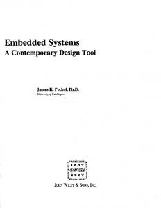
superset of HRELTL that encompasses first-order constructs to represent classes of objects and their relationships. The extension enriches the representation power of the discrete part of the specification, and therefore it is orthogonal to the hybrid aspects of the language. The techniques used to handle objects and first-order constraints are described in [10]. We implemented the translation from linear HRELTL to RELTL in an extended version of the N U SMV [9] model checker that interfaces with the MathSAT [5] SMT solver. For an RELTL formula φ, we use N U SMV to compile φ into an equivalent FTS Sφ . Then, we check the language non-emptiness of Sφ by submitting the corresponding BMC problem to the MathSAT SMT solver. We ran the experiments on a 2.20GHz Intel Core2 Duo Laptop equipped with 2GB of memory running Linux version 2.6.24. All the data and binaries necessary to reproduce the results here presented are available at http://es.fbk.eu/people/tonetta/tests/cav09/. We extracted from the fragment of the ETCS specification a set of requirements that falls in HRELTL and that are relevant for their hybrid aspects. This resulted in a case study consisting of 83 HRELTL formulas, with 15 continuous variables, of which three are timers and two are stop watches. An excerpt of the ETCS specification in HRELTL format is reported in Sec. D. We first checked whether the specification is consistent, i.e. if it is satisfiable (SAT). Then, we validated the formalization with 3 different scenarios (SCEN {1,2,3}), checking the satisfiability of the conjunction of the specification with a formula that represents some assumptions on the evolution of the variables. In all cases, the tool generated a trace proving the satisfiability of the formulas. We then asked the tool to generate witness traces of different increasing lengths k (10, 20, and 30 respectively). We obtained the results reported in Fig. 3(a). In the table we report also the size, in terms of number of variables and number of fairness conditions of the FTS we submit to underlying verification tool. (We use #r,#b,#f with the meaning, r Real variables, b Boolean variables, and f fairness conditions.) Fig. 3(b) also reports some curves that we can extract from the trace generated by the tool. These curves are the same that are manually depicted in ETCS (Fig. 1(b)). The fact that the automated generated traces resemble the ones inserted in the requirements document makes us more confident that the requirements captures what the designers have in mind.

8

Related Work

To the best of our knowledge, this is the first attempt to generalize requirements validation to the case of hybrid domains. The work most closed to the current paper is described in [13], where LTL with continuous and hybrid semantics is compared with the discrete semantics. It is proved that a positive answer to the model checking problem and to the validity problem with the discrete semantics implies a positive answer to the corresponding problem in the continuous semantics. The properties of finite variability and sampling invariance are introduced. Notably, the hybrid semantics of the logic relies on the hybrid traces accepted by a hybrid system (while our definition is independent). 12

Name: SAT SAT SAT SCEN SCEN SCEN SCEN SCEN SCEN SCEN SCEN SCEN

1 1 1 2 2 2 3 3 3

Sat k #r,#b,#f Mem (MB) Y 10 56,310,17 74.8 Y 20 56,310,17 122.4 Y 30 56,310,17 173.0 Y 10 56,312,19 75.4 Y 20 56,312,19 123.1 Y 30 56,312,19 174.3 Y 10 56,312,19 76.8 Y 20 56,312,19 127.1 Y 30 56,312,19 180.0 Y 10 56,323,18 75.9 Y 20 56,323,18 122.5 Y 30 56,323,18 173.3

Time (sec) 11.38 55.38 141.20 15.00 78.09 190.73 17.56 78.26 270.59 19.16 52.52 147.97

7

P_limit W_limit SBI_limit SBD_limit EBI_limit EBD_limit

6 5 4 3 2 1 0 0

1

2

3

4

5

6

7

8

9

(a)

(b) Fig. 3. The results of the experimental evaluation.

Besides [13], our work is also inspired by the ones of [23, 26, 22]. [23, 26] face the problem of the observability of predicates during continuous evolutions, and define phase transition systems, which are a symbolic version of hybrid automata. [22] formally defines a continuous semantics for LTL without next operator and derivatives. In all these works, there is no attempt to solve the satisfiability problem for LTL with the continuous semantics. Many logics have been introduced to describe properties of timed systems (see [3, 4] for a survey), but none of them can force the continuity of functions, because the semantics is discrete, though in some cases even a dense time domain is considered. Hybrid systems [26, 19] assume that some functions are continuous but the logic used to express the properties is discrete. In [21, 17], a translation from dense time to discrete time is proposed for a particular class of specifications, but only discrete semantics is considered. In [29], the discretization of hybrid systems is obtained with an over-approximation, while our translation produces an equi-satisfiable discrete formula. In [18], a framework for specifying requirements of hybrid systems is proposed. However, the techniques are model based, and the requirements are formalized in a tabular notation, which can be seen as a symbolic representation of an automaton. In [28], a hybrid dynamic logic is proposed for the verification of hybrid systems and it was used to prove safety properties for ETCS. The approach is still model-based since the description of the system implementation is embedded in the logical formula. The regular expression operations are used to define hybrid programs, that represent the hybrid systems. Properties of hybrid programs are expressed with the modalities of firstorder dynamic logic. As in RELTL, we use regular expressions with a linear semantics. Moreover, the constraints on the continuous evolution are part of the requirements rather than the system description. As explained in Sec. 2, our approach to the validation of ETCS specifications is property-based. In [2, 19], linear hybrid automata are defined and a symbolic procedure is proposed to check their emptiness. Besides the different property-based approach that we propose, our techniques differ in the following points. First, instead of a finite set of states, the discrete modes are represented by the infinite (uncountable) set of assignments to the discrete variables. Second, instead of fix-point computations where the image is 13

based on the quantifier elimination in the theory of Reals, we propose a BMC-based approach with a quantifier-free encoding (this is accomplished by forcing each step to move in a convex region). Related to the encoding of invariants that hold in a continuous evolution, also [30] faces the problem of concave conditions, and splits concave time conditions into convex segments. The condition (3) of our translation has the purpose to split the trace into convex regions in an analogue way. In [24], a continuous semantics to a temporal logic which does not consider next operators and derivatives is presented. The paper addresses the problem of monitoring temporal properties of circuits with continuous signals. On a different line of research, Duration Calculus (DC) [7] specifies requirements of real-time systems with predicates over the integrals of Boolean functions over finite intervals of time. Extensions of DC such as Extended Duration Calculus [8] can specify properties over continuous and differentiable functions. DC has been used to specify properties for ETCS [16]. Similarly to DC, Hybrid Temporal Logic (HTL) [20] uses the “chop” operator to express the temporal succession and can express temporal constraints on the derivatives of dynamic functions. Both DC and HTL interpret formulas over intervals of time (rather than infinite sequences of intervals). On the contrary, HRELTL is based on RELTL, which has been consolidated as specification language at the industrial level. HRELTL has the advantage to allow the reuse of requirements analysis techniques for RELTL.

9

Conclusions and future work

In this paper, we tackled the problem of validating requirements for hybrid systems. We defined a new logic HRELTL, that allows to predicate over properties of hybrid traces. Then, we showed that the satisfiability for the linear fragment of HRELTL can be reduced to an equi-satisfiable problem for RELTL over discrete traces. HRELTL was used for modeling in a real-world project aiming at the validation of a subset of the ETCS specification. The validation showed that the temporal requirements of ETCS can be formalized with HRELTL, and the experimental evaluation we carried out showed the practicality of the analysis, based on the use of SMT techniques. As future work, we will enhance the scalability of the satisfiability procedure, by means of incrementality, lemmas on demand, and abstraction-refinement techniques. We will also consider alternative ways to deal with nonlinear constraints.

References 1. The PROSYD project on property-based system design, 2007. http://www.prosyd.org. 2. R. Alur, C. Courcoubetis, T. A. Henzinger, and P-H. Ho. Hybrid Automata: An Algorithmic Approach to the Specification and Verification of Hybrid Systems. In Hybrid Systems, pages 209–229, 1992. 3. R. Alur and T. A. Henzinger. Logics and Models of Real Time: A Survey. 1992. 4. R. Alur and T. A. Henzinger. Real-Time Logics: Complexity and Expressiveness. Inf. Comput., 104(1):35–77, 1993. 5. R. Bruttomesso, A. Cimatti, A. Franz´en, A. Griggio, and R. Sebastiani. The MathSAT 4 SMT Solver. In CAV, pages 299–303, 2008.

14

6. D. Bustan, A. Flaisher, O. Grumberg, O. Kupferman, and M.Y. Vardi. Regular Vacuity. In CHARME, pages 191–206, 2005. 7. Z. Chaochen, C. A R. Hoare, and A. P. Ravn. A calculus of durations. Inf. Process. Lett., 40(5):269–276, 1991. 8. Z. Chaochen, A. P. Ravn, and M. R. Hansen. An extended duration calculus for hybrid real-time systems. In Hybrid Systems, pages 36–59, 1992. 9. A. Cimatti, E.M. Clarke, F. Giunchiglia, and M. Roveri. N U SMV: a new Symbolic Model Verifier. In CAV 1999, volume 1633 of LNCS, 1999. 10. A. Cimatti, M. Roveri, A. Susi, and S. Tonetta. Object models with temporal constraints. In SEFM 2008, pages 249–258. IEEE press, 2008. 11. A. Cimatti, M. Roveri, and S. Tonetta. Symbolic Compilation of PSL. IEEE Trans. on CAD of Integrated Circuits and Systems, 27(10):1737–1750, 2008. 12. K. Claessen. A coverage analysis for safety property lists. In FMCAD, pages 139–145. IEEE, 2007. 13. L. de Alfaro and Z. Manna. Verification in Continuous Time by Discrete Reasoning. In AMAST, pages 292–306, 1995. 14. ERTMS/ETCS — Baseline 3: System Requirements Specifications. SUBSET-026-1, i3.0.0, 2008. http://www.era.europa.eu/core/ertms/Pages/FirstETCSSRS300.aspx. 15. H. Eveking, M. Braun, M. Schickel, M. Schweikert, and V. Nimbler. Multi-level assertionbased design. In MEMOCODE, pages 85–86. IEEE, 2007. 16. J. Faber and R. Meyer. Model checking data-dependent real-time properties of the european train control system. In FMCAD, pages 76–77, 2006. 17. C. A. Furia, M. Pradella, and M. Rossi. Automated Verification of Dense-Time MTL Specifications Via Discrete-Time Approximation. In FM, pages 132–147, 2008. 18. C. L. Heitmeyer. Requirements Specifications for Hybrid Systems. In Hybrid Systems, pages 304–314, 1995. 19. T. A. Henzinger. The Theory of Hybrid Automata. In LICS, pages 278–292, 1996. 20. T. A. Henzinger, Z. Manna, and A. Pnueli. Towards refining temporal specifications into hybrid systems. In Hybrid Systems, pages 60–76, 1992. 21. T. A. Henzinger, Z. Manna, and A. Pnueli. What Good Are Digital Clocks? In ICALP, pages 545–558, 1992. 22. A. Kapur. Interval and point-based approaches to hybrid system verification. PhD thesis, Stanford, CA, USA, 1998. 23. O. Maler, Z. Manna, and A. Pnueli. From Timed to Hybrid Systems. In REX Workshop, pages 447–484, 1991. 24. O. Maler, D. Nickovic, and A. Pnueli. Checking Temporal Properties of Discrete, Timed and Continuous Behaviors. In Pillars of Computer Science, pages 475–505, 2008. 25. Z. Manna and A. Pnueli. The Temporal Logic of Reactive and Concurrent Systems: Specification. Springer-Verlag, 1992. 26. Z. Manna and A. Pnueli. Verifying Hybrid Systems. In Hybrid Systems, pages 4–35, 1992. 27. I. Pill, S. Semprini, R. Cavada, M. Roveri, R. Bloem, and A. Cimatti. Formal analysis of hardware requirements. In DAC, pages 821–826, 2006. 28. A. Platzer. Differential Dynamic Logic for Verifying Parametric Hybrid Systems. In TABLEAUX, pages 216–232, 2007. 29. A. Tiwari. Abstractions for hybrid systems. Formal Methods in System Design, 32(1):57–83, 2008. 30. F. Wang. Time-Progress Evaluation for Dense-Time Automata with Concave Path Conditions. In ATVA, pages 258–273, 2008.

15

A

Abbreviations

We use the following standard abbreviations: >= ˙ p ∨ ¬p ϕ1 ∨ ϕ2 = ˙ ¬(¬ϕ1 ∧ ¬ϕ2 ) Fϕ= ˙ >Uϕ ϕ1 V ϕ2 = ˙ ¬(¬ϕ1 U ¬ϕ2 ) r+ = ˙ r; r∗

B

STEP = ˙ (pnext ∨ pnext ) ϕ1 → ϕ2 = ˙ ¬ϕ1 ∨ ϕ2 Gϕ= ˙ ¬F ¬ϕ ϕ1 W ϕ2 = ˙ ϕ1 U ϕ2 ∨ G ϕ1 r |→ ϕ = ˙ ¬r ♦→ ¬ϕ

A temporal logic for hybrid traces

Theorem 1 (Finite variability). Given a formula φ, for every hybrid trace hf , Ii there 0 0 exists another hybrid trace hf , I i which is a sampling refinement of hf , Ii and ground for φ. Proof. The theorem is guaranteed by the analyticity of every function fi and the analyticity of the functions used to form predicates. Since the composition of analytic functions is analytic, the truth value of a predicate cannot change infinitely many times in a given interval. Formally, given a predicate p occurring in φ, p is in the form g ./ 0, with g : Σ → R analytic. For every i ∈ N, fi : R → Σ is piecewise analytic. Therefore the composition g · fi is a real analytic function. Thus, the function is either constantly zero or has a finite number of zeros in Ii . Let such points be the sequence t1i , t2i , ..., tni i . Finally, consider the sampling refinement of hf , Ii of hf, Ii that splits every open interval Ii = (ti , ti+1 ) into (ti , t1i ), [t1i , t1i ], (t1i , t2i ), ..., (tni i , ti+1 ). Note that for all i, for all predicate p occurring in φ, suppose p is in the form g ./ 0, then the interpretation of g in I i either is constantly zero or is never zero. Since g is continuous, the interpretation of p in I i is constant. Therefore hf , Ii is ground for φ. 0

0

Lemma 1. Given two hybrid traces hf , Ii and hf , I i, if hf , Ii is ground for φ and 0 0 0 0 hf , I i µ hf , Ii, then, for all i ∈ N, for all j ∈ µi , hf , Ii, i |= p iff hf , I i, j |= p. 0

0

Proof. If Ii = [t, t] then Ij = Ii and thus hf , Ii, i |= p iff hf , I i, j |= p. Suppose Ii = (t, t0 ) then either Ij = (t1 , t2 ) with t ≤ t1 < t2 ≤ t0 or Ij = [t1 , t1 ] with t < t1 < t0 . Suppose Ij = (t1 , t2 ). – If p contains only variables in V , σ, i |= p iff, for all t ∈ Ii , fi (t) |= p. If, for all t ∈ Ii , fi (t) |= p, then, for all t ∈ Ij , fj (t) |= p since Ij ⊆ Ii and fj = fi . If, for all t ∈ Ij , fj (t) |= p, then, for all t ∈ Ii , fi (t) |= p since hf , Ii is ground for p. – If p contains variables in VNEXT then σ, i 6|= p and σ 0 , j 6|= p. – If p contains only variables in V , σ, i |= p iff, for all t ∈ Ii , fi (t), f˙i (t)− |= p and fi (t), f˙i (t) + − |= p. If, for all t ∈ Ii , fi (t), f˙i (t)− |= p, then, for all t ∈ Ij , fj (t), f˙j (t)− |= p since Ij ⊆ Ii and fj = fi f˙i (t)− = f˙j (t)− . If, for all t ∈ Ij , fj (t), f˙j (t)− |= p, then, for all t ∈ Ii , fi (t), f˙i (t)− |= p since hf , Ii is ground for p. The same applies to right derivative. 16

0

0

Lemma 2. If hf , Ii is a trace ground for φ and hf , I i is a sampling refinement of hf , Ii by the partitioning µ, then for all i, j ∈ N, for all i0 ∈ µi , j 0 ∈ µj , for all SERE 0 0 r that occur in φ, hf , Ii, i, j |= r iff hf , I i, i0 , j 0 |= r. Proof. We prove the lemma by induction on the definition of r: – If r = p, for some predicate p, and i = j, then i0 and j 0 are indexes of the same 0 0 continuous evolution. Since hf , Ii is ground, hf , Ii, i0 |= p iff hf , I i, j 0 |= p. 0 0 Thus, hf , Ii, i, j |= p iff hf , I i, i0 , j 0 |= p. Suppose now r = p and i < j. By definition of sampling refinement, there are no discrete steps between i and j iff there are no discrete steps between i0 and j 0 . Moreover, since the trace is ground for p, hf , Ii, k |= p for all k, i ≤ k ≤ j, iff hf , Ii, k |= p for all k 0 , i0 ≤ k 0 ≤ j 0 . – If r = , then hf , Ii, i, j |= r iff i > j. Though, i > j iff i0 > j 0 . – Suppose r = r1 ∗. This case is proved by induction on j − i. As for the base case, i > j iff i0 > j 0 . For the inductive hypothesis on r, hf, Ii, i, j |= r, iff hf , Ii, i0 , j 0 |= r for all i, j ∈ N, for all i0 ∈ µi , j 0 ∈ µj . Thus, if i ≤ k < j, hf , Ii, i, k |= r, hf , Ii, k + 1, j |= r∗ iff hf , Ii, i0 , k 0 |= r, hf , Ii, k 0 + 1, j 0 |= r∗. Finally, note that if Ik0 = Ik0 +1 = [t, t], then k 0 ∈ µk iff k 0 + 1 ∈ µk0 +1 . – The cases r = r1 ; r2 and r = r1 : r2 are similar to previous one. – The cases r1 |r2 and r1 &&r2 can be proved directly from the inductive hypothesis. 0

0

Lemma 3. If two hybrid traces hf , Ii and hf , I i are ground for a formula φ and they 0 0 are one a sampling refinement of the other, then hf , Ii |= φ iff hf , I i |= φ. Proof. We prove by induction on φ that, for all i ∈ N, for all j ∈ µi , hf , Ii, i |= φ iff 0 0 hf , I i, j |= φ. – Suppose p is a predicate; then the claim is true by Lemma 1. – Suppose φ is in the form ¬φ1 , φ1 ∧ φ2 , X φ1 , φ1 U φ2 . Then the claim follows directly from the inductive hypothesis. – Suppose φ is in the form r ♦→ φ1 . Then for Lemma 2, hf, Ii, i, k |= r, iff hf , Ii, i0 , k 0 |= r for all i, k ∈ N, for all i0 ∈ µi , k 0 ∈ µk . Thus, if i ≤ k, hf , Ii, i, k |= r, hf , Ii, k |= φ1 then hf , Ii, j, k 0 |= r, hf , Ii, k 0 |= φ1 for some k 0 ∈ µk (since µk is not empty). If hf , Ii, j, k 0 |= r, hf , Ii, k 0 |= φ1 for some k 0 ∈ µk , then i ≤ k, hf , Ii, i, k |= r, hf , Ii, k |= φ1 . 0

0

Theorem 2 (Sample invariance). If hf , I i is a sampling refinement of hf , Ii, then the two hybrid traces satisfy the same formulas. 0

0

Proof. Given a formula φ, for Theorem 1, both traces hf , Ii and hf , I i have a sam0 0 pling refinement ground for φ, named resp. hf G , I G i and hf G , I G i. Since hf , Ii µ1 0 0 hf , I i, hf G , I G i µ2 hf , Ii, there exists a refinement µ3 such that hf G , I G i µ3 0 0 0 0 0 00 00 0 hf , I i. Since hf G , I G i µ4 hf , I i, there exists a sampling refinement hf , I i that 0 0 merges the splitting of µ3 and µ4 , thus refining both hf G , I G i and hf G , I G i. For Lemma 00 00 0 0 3, hf G , I G i |= φ iff hf , I i |= φ iff hf G , I G i |= φ. 17

C

Reduction to discrete semantics

In this section we give the formal semantics of RELTL and the proofs of our translation. Given a predicate p and a state s, we assume that the relation s |= p defining when the state satisfies the predicate is given. Definition 12 (SERE semantics). – σ, i, j |= p iff, i = j, and σi |= p; – σ, i, j |=  iff i > j; – σ, i, j |= r[*] iff i > j or σ, i, j |= r, or there exists k, i ≤ k < j, such that σ, i, k |= r, σ, k + 1, j |= r[*]; – σ, i, j |= r1 ; r2 iff σ, i, j |= r1 , σ, j + 1, j |= r2 , or σ, i, i − 1 |= r1 , σ, i, j |= r2 , or there exists k, i ≤ k < j, such that σ, i, k |= r1 , σ, k + 1, j |= r2 ; – σ, i, j |= r1 : r2 iff there exists k, i ≤ k ≤ j, such that σ, i, k |= r1 , σ, k, j |= r2 ; – σ, i, j |= r1 | r2 iff σ, i, j |= r1 or σ, i, j |= r2 ; – σ, i, j |= r1 && r2 iff σ, i, j |= r1 and σ, i, j |= r2 . Definition 13 (RELTL semantics). – σ, i |= p iff σi |= p; – σ, i |= ¬φ iff σ, i 6|= φ; – σ, i |= φ ∧ ψ iff σ, i |= φ and σ, i |= ψ; – σ, i |= X φ iff σ, i + 1 |= φ; – σ, i |= φ U ψ iff, for some j ≥ i, σ, j |= ψ and, for all i ≤ k < j, σ, k |= φ; – σ, i |= r ♦→ φ iff, there exists j ≥ i, such that σ, i, j |= r and σ, j |= φ. The following three lemmas prove that if σ is a hybrid trace than Ω(σ) |= ψι ∧ ψDER ∧ ψP REDφ ∧ ψVD . Vice versa, if σ |= ψι ∧ ψDER ∧ ψVD , then Υ (σ) is a hybrid trace. Lemma 4. If σ a hybrid trace, then Ω(σ) |= ψι . If σ |= ψι , then the intervals of Υ (σ) are adjacent and cover R+ . Proof. Suppose σ is a hybrid trace. Then I0 = [0, 0] and s0 (ι) = >. If Ii = Ii+1 = [t, t] then si (ι) = si+1 (ι) = > and si (δt ) = 0. If Ii = [t, t] and Ii+1 = (t, t0 ) then si (ι) = >, si (δt ) = (t0 − t)/2 > 0 and si+1 (ι) = ⊥. If Ii = (t, t0 )Sand Ii+1 = [t, t] then si (ι) = ⊥, si (δt ) = (t0 − t)/2 > 0 and si+1 (ι) = >. Finally, i∈N Ii = R+ so that the sequence {ti }i∈N must be divergent. Then, for the Chauchy’s condition, there exists α = s0 (ζ) > 0 such that for all i ∈ N, there exists j ≥ i such that ti+1 − ti ≥ α. and thus sj (δt ) ≥ sj (ζ). Suppose σ |= ψι . Then I0 = [0, 0] and there exists α = s0 (ζ) > 0 such that for all i ∈ N, there exists j ≥ i such thatSsj (δt ) ≥ sj (ζ), and thus ti+1 − ti ≥ α. Hence, t0 = 0 and {ti }i∈N diverges, and so i∈N Ii = R+ . If si (ι) = si+1 (ι) = > then Ii = Ii+1 = [ti , ti ]. If si (ι) = >, and si+1 (ι) = ⊥ then Ii = [ti , ti ] and Ii+1 = (ti , ti+2 ). If si (ι) = ⊥, and si+1 (ι) = > then Ii = (ti−1 , ti+1 ) and Ii+1 = [ti+1 , ti+1 ]. Lemma 5. If σ a hybrid trace, then Ω(σ) |= ψDER . If σ |= ψDER , then for all i ∈ N, for all v ∈ VC , if Ii = (t, t0 ) then fi (t) = fi−1 (t), fi (t0 ) = fi+1 (t0 ). 18

Proof. Suppose σ is a hybrid trace. If si (δt ) > 0 ∧ ι then Ii = [t, t] and Ii+1 = v v v (ti ) = fiv (ti ), (ti ))/(ti+1 − ti ). Since fi+1 (ti+1 ) − fi+1 (t, t0 ) and si+1 (v˙ l ) = (fi+1 si+1 (v) − si (v) = δt × si+1 (v˙ l ). v If si (δt ) > 0 ∧ ¬ι then Ii = (t, t0 ) and Ii+1 = [t0 , t0 ] and si (v˙ r ) = (fi+1 (ti+1 ) − v v v fi+1 (ti ))/(ti+1 − ti ). Since fi+1 (ti ) = fi (ti ), si+1 (v) − si (v) = δt × si (v˙ r ). Now, suppose σ |= ψDER . If Ii = [t0 , t0 ] and Ii+1 = (t0 , t) (first case of Equation 2), si+1 (v) − si (v) = v si (δt ) × si+1 (v˙ l ). By Definition 11, fi+1 (t) = si+1 (v) − si+1 (v˙ l ) × (ti+1 − t) if v 0 t ≤ ti+1 . In particular, fi+1 (t ) = si+1 (v) − si+1 (v˙ l ) × si (δt ). Substituting, we get v fi+1 (t0 ) = si (v). Since, by Definition 11, si (v) = fiv (t0 ), the result holds. If Ii = (t, t0 ) and Ii+1 = [t0 , t0 ] (second case of Equation 2), si+1 (v) − si (v) = si (δt ) × si (v˙ r ). By Definition 11, fiv (t) = si (v) + si (v˙ r ) × (t − ti ) if t > ti . In particular, fiv (t0 ) = si (v) + si (v˙ r ) × si (δt ). Substituting, we get fiv (t0 ) = si+1 (v). v (t0 ), the result holds. Since, by Definition 11, si+1 (v) = fi+1 Lemma 6. If σ a hybrid trace, then If σ is ground for φ, Ω(σ) |= ψP REDφ . If σ |= ψP REDφ , then Υ (σ) is ground for φ. Proof. Suppose Ii = [t, t], Ii+1 = (t, t0 ), and Ω(σ), i 6|= NEXT(p= ) → p= . Since p= is an open set and fi+1 is continuous, by topology f −1 (p= ) must be open. Thus there exist t00 ∈ (t, t0 ) such that fi+1 (t00 ) |= p= , which violates the hypothesis that σ is ground. The case p= → NEXT(p= ) is similar. Suppose Ω(σ) does not satisfy (p< → ¬X p> ) for some p ∈ P RED, then by Bolzano’s theorem, we can pick a point in the interval such that p= holds, which violates the hypothesis that σ is ground. The case in which Ω(σ) does not satisfy (p> → ¬X p< ) is similar. Suppose σ |= ψP REDφ . Suppose Ii = (t, t0 ) and fi (ti ) |= p= then, by hypothesis, fi (t) |= p= and fi (t0 ) |= p= . Since fi is linear over [t, ti ] and [ti , t0 ], and p= is convex, then fi (t00 ) |= p= for all t00 ∈ (t, t0 ). Suppose fi (ti ) |= p< then, by hypothesis, fi (t) |= ¬p> and fi (t0 ) |= ¬p> . Since fi is linear over [t, ti ] and [ti , t0 ], and p= is convex, then fi (t00 ) |= p< for all t00 ∈ (t, t0 ). The case for p> is similar. We conclude that Υ (σ) is ground. Lemma 7. If σ a hybrid trace, then Ω(σ) |= ψVD . If σ |= ψDER ∧ ψVD , then for all v ∈ VD , fiv is constant. Proof. For all v ∈ VD , v is constant when δt > 0 and thus Ω(σ) |= ψVD . If σ |= ψDER ∧ ψVD , if σi (δt ) > 0 then for all v ∈ VD , σi (v˙ l ) and σi (v˙ r ) are zero, and therefore fiv is constant. Lemma 8. If σ is ground for a predicate p, σ, i |= p iff Ω(σ), i |= τa0 (p). Proof. – If σ, i |= pcurr then, for all t ∈ Ii , fi (t) |= pcurr and in particular fi (ti ) |= pcurr , i.e., si |= pcurr . Vice versa, if si |= pcurr , then fi (ti ) |= pcurr , and since σ is ground for pcurr , for all t ∈ Ii , fi (t) |= pcurr . – σ, i |= pnext iff Ii = Ii+1 = [t, t] and fi (t), fi+1 (t) |= pnext , i.e. si (t), si+1 (t) |= pnext and σ, i |= δt = 0. 19

– If σ, i |= pder and Ii = (t, t0 ), then, for all t ∈ Ii , fi (t), f˙i (t) |= pder . In particular fi (ti ), f˙i (ti ) |= pder . By the mean value theorem there is a point t in (t, (t + t0 )/2) such that f˙i (t) = si (v˙ l ) and another point in ((t+t0 )/2, t0 ) such that f˙i (t) = si (v˙ r ). In both cases, since g contains only discrete variables, fi (ti ), f˙i (t) |= pder . Vice versa, if fi (ti ), f˙i (ti ) |= pder , then there exists t as above and since σ is ground for pder , for all t ∈ Ii , fi (t), f˙i (t) |= pder . If Ii = [t, t], then fi (t), f˙i (t)− |= pder and fi (t), f˙i (t)+ |= pder iff si |= pder [v˙ l /DER(v)] ∧ pder [v˙ r /DER(v)]. Lemma 9. If σ is ground for a SERE r, then σ, i, j |= r iff Ω(σ), i, j |= τr0 (r). Proof. – σ, i, j |= p iff, for all k, i ≤ k < j, there is no discrete step at k (Ik 6= Ik+1 ), and, for all k, i ≤ k ≤ j, σ, k |= p; thus, σ, i, j |= p, iff for all k, i ≤ k < j, Ω(σ), k |= δt > 0, and, for all k, i ≤ k ≤ j, Ω(σ), k |= τa0 (p) (for Lemma 8); – σ, i, j |=  iff i > j iff Ω(σ), i, j |= ; – σ, i, j |= r[*] iff i > j, or σ, i, j |= r, or there exists a discrete step at k (Ik = Ik+1 ), i ≤ k < j, such that σ, i, k |= r, σ, k + 1, j |= r[*]; the first case holds iff Ω(σ), i, j |= ; the second case iff there exist n discrete steps at k1 , k2 , . . . kn such that Iki = Iki +1 and σ, i, k1 |= r, σ, k1 , k2 |= r, ... σ, kn , j |= r iff (for inductive hypothesis) Ω(σ), i, k1 |= τr0 (r), Ω(σ), k1 + 1, k2 |= τr0 (r), ... Ω(σ), kn + 1, j |= τr0 (r), and Ω(σ), k1 |= δt = 0, Ω(σ), k1 + 1, k2 |= δt = 0, ... Ω(σ), kn + 1, j |= δt = 0; – σ, i, j |= r1 ; r2 iff σ, i, j |= r1 , σ, j + 1, j |= r2 (i.e., r2 accepts the empty word), or σ, i, i − 1 |= r1 , σ, i, j |= r2 (i.e., r1 accepts the empty word), or there exists a discrete step at k (Ik = Ik+1 ), i ≤ k < j, such that σ, i, k |= r1 , σ, k + 1, j |= r2 ; the first case holds, by induction, iff Ω(σ), i, j |= r1 , Ω(σ), j + 1, j |= r2 and thus iff Ω(σ), i, j |= τr0 (r1 ) ; { && τr0 (r2 )}; the second case holds, by induction, iff Ω(σ), i, i − 1 |= r1 , Ω(σ), i, j |= r2 and thus iff Ω(σ), i, j |= { && τr0 (r1 )} ; τr0 (r2 ); the third case holds, by induction, iff Ω(σ), i, i − 1 |= r1 , Ω(σ), i, j |= r2 and thus iff Ω(σ), i, j |= { && τr0 (r1 )} ; τr0 (r2 ); – σ, i, j |= r1 : r2 iff there exists a discrete step at k (Ik = Ik+1 ), i ≤ k ≤ j, such that σ, i, k |= r1 , σ, k, j |= r2 iff (by inductive hypothesis) Ω(σ), i, k |= τr0 (r1 ), Ω(σ), k, j |= τr0 (r2 ), and Ω(σ), k |= δt = 0, – σ, i, j |= r1 | r2 iff σ, i, j |= r1 or σ, i, j |= r2 iff (by inductive hypothesis) Ω(σ), i, j |= τr0 (r1 ) or Ω(σ), i, j |= τr0 (r2 ); – σ, i, j |= r1 && r2 iff σ, i, j |= r1 and σ, i, j |= r2 iff (by inductive hypothesis) Ω(σ), i, j |= τr0 (r1 ) and Ω(σ), i, j |= τr0 (r2 ). Lemma 10. If σ is ground for φ, then σ, i |= φ iff Ω(σ), i |= τ 0 (φ). Proof. – σ, i |= p iff Ω(σ), i |= p for Lemma 8; – σ, i |= ¬φ iff σ, i 6|= φ iff Ω(σ), i 6|= τ 0 (φ) (by inductive hypothesis); – σ, i |= φ ∧ ψ iff σ, i |= φ and σ, i |= ψ iff Ω(σ), i |= τ 0 (φ) and Ω(σ), i |= τ (ψ); – σ, i |= X φ iff there is a discrete step at i (Ii = Ii+1 ), and σ, i + 1 |= φ iff Ω(σ), i |= δt = 0 and Ω(σ), i |= τ 0 (X φ); – σ, i |= φ U ψ iff, for some j ≥ i, σ, j |= ψ and, for all i ≤ k < j, σ, k |= φ iff Ω(σ), j |= τ (ψ) and, for all i ≤ k < j, Ω(σ), k |= τ 0 (φ); 20

– σ, i |= r ♦→ φ iff, there exists a discrete step at j ≥ i (Ij = Ij+1 ) such that σ, i, j |= r, and σ, j |= φ iff Ω(σ), i, j |= τr0 (r), and Ω(σ), j |= τ 0 (φ). Lemma 11. If σ |= ψι ∧ ψDER ∧ ψP REDφ ∧ ψVD , σ, i |= τ 0 (φ) iff Υ (σ), i |= φ. Proof. – If σ, i |= pcurr then fi (ti ) |= pcurr , and since Υ (σ) is ground, for all t ∈ Ii , fi (t) |= pcurr . – If σ, i |= (δt = 0) ∧ pnext , then Ii = Ii+1 = [t, t] and fi (t), fi+1 (t) |= pnext . – If σ, i |= pder [v˙ l /DER(v)] ∧ pder [v˙ r /DER(v)], then, for all t < ti , fi (t), f˙i (t) |= pder because f˙i (t) = v˙ l , and, for all t > ti , fi (t), f˙i (t) |= pder because f˙i (t) = v˙ r . – The other cases result directly from the inductive hypothesis similarly to Lemmas 9 and 10. Theorem 3 (Equi-satisfiability). If hf , Ii is ground for φ and hf , Ii |= φ, then Ω(hf , Ii) |= τ (φ). If σ is a discrete trace such that σ |= τ (φ), then Υ (σ) |= φ and Υ (σ) is ground for φ. Thus φ and τ (φ) are equi-satisfiable. Proof. Suppose σ |= φ. Then for Lemmas 4, 5, 6, and 7, Ω(σ) |= ψι ∧ψDER ∧ψP REDφ ∧ ψVD . For Lemma 10, Ω(σ) |= τ 0 (φ). Thus, Ω(σ) |= τ (φ). Suppose σ |= τ (φ). Then σ |= τ 0 (φ), and, for Lemma 11, Υ (σ) |= φ. Finally, for Lemmas 4, 5, 6, and 7, Υ (σ) is a hybrid trace.

D

ETCS case study in HRELTL

----------------------------- Background assumptions ------------------------------ declaration of train front end VAR train.front_end: continuous; -- the train front end does not change during discrete steps FORMULA G ! ( next(train.front_end)!=train.front_end ) -- declaration of train min and max safe_front_end VAR train.min_safe_front_end: continuous; train.max_safe_front_end: continuous; -- relation between train front_end and min_safe_front_end FORMULA G ( train.front_end>=train.min_safe_front_end ) -- relation between train front_end and max_safe_front_end FORMULA G ( train.front_end next(receive_MA)=FALSE ) -- declaration of MA message contents FROZENVAR MA_message.time_stamp: real; -- declaration of passage time over the first balise of the current -- balise group FROZENVAR current_balise_group.first_balise.passage_time_stamp: real; -------------------------- Scenario conditions ------------------------------------------------- ETCS requirements ------------------------- 3.8 Movement authority -- 3.8.1 Characteristics of a MA -- 3.8.1.1 The following characteristics can be used in a Movement -Authority (see Figure 17: -- Structure of an MA): -- a) The End Of Authority (EOA) is the location to which the train is -authorized to move. VAR eoa: real;

22

FORMULA G ( eoa>=0 ) -- b) The Target Speed at the EOA is the permitted speed at the EOA; -when the target speed is not zero, the EOA is called the Limit -of Authority (LOA). This target speed can be time limited. VAR eoa_target_speed: real; eoa_target_speed_timeout: real; FORMULA G ( eoa_target_speed >=0 ) FORMULA G ( (train.front_end=eoa) -> train.speedeoa ) FORMULA G ( (ol=0 & train.front_end>dp) -> hazard ) -- d) The end of an overlap (if used in the existing interlocking -system) is a location beyond the Danger Point that can be reached -by the front end of the train without a risk for a hazardous -situation. This additional distance is only valid for a defined -time. VAR end_ol: real; FORMULA G ( end_ol>=dp ) FORMULA G ( ol = end_ol - dp ) FORMULA G ( (train.front_end>end_ol) -> hazard ) -- e) A release speed is a speed under which the train is allowed to -run in the vicinity of the EOA, when the target speed is zero. One -release speed can be associated with the Danger Point, and another

23

-one with the overlap. Release speed can also be calculated on-board -the train (see section 3.13.7). VAR eoa_release_speed: real; eoa_vicinity: real; dp_release_speed: real; dp_vicinity: real; ol_release_speed: real; ol_vicinity: real; FORMULA G ( ( train.front_end>=(eoa - eoa_vicinity) & eoa_target_speed=0) -> train.speed=(dp - dp_vicinity) & ol=0) -> train.speed=(ol - ol_vicinity) & ol>0) -> train.speed=0) FORMULA G (section[1].start der(section[1].timer)=1 ) FORMULA G ( (level=2 & receive_MA) -> ( next(section[1].timer)=MA_message.time_stamp & next(section[1].timer_stop)=FALSE ) ) FORMULA G ( (level=1 & receive_MA) -> ( next(section[1].timer)= current_balise_group.first_balise.passage_time_stamp & next(section[1].timer_stop)=FALSE ) ) FORMULA G ( endsection.timer_stop -> der(endsection.timer)=0 ) FORMULA G ( !endsection.timer_stop -> der(endsection.timer)=1 ) FORMULA G ( (level=2 & receive_MA) -> ( next(endsection.timer)=MA_message.time_stamp & next(endsection.timer_stop)=FALSE ) ) FORMULA G ( (level=1 & receive_MA) -> ( next(endsection.timer)= current_balise_group.first_balise.passage_time_stamp & next(endsection.timer_stop)=FALSE ) ) -- 3.8.4.2.2 When the time out has expired, the EOA shall be withdrawn -to the entry point of the revoked section. FORMULA G ( section[1].timer ( section[1].timer ( der(train.front_end)>0 W ( der(train.front_end)=0 & next(ol)=0 ) ) ) -- 3.8.4.5 -- 3.8.4.5.1 ----

Supervised Location The Supervised Location shall be defined on board as; a) the end of overlap (if any and before time-out). b) if not, the Danger Point (if any). c) if not, the End Of Authority.

VAR SL: real; FORMULA G ( SL=(case ol>0: end_ol; dp>eoa: dp; 1: eoa; esac) ) -- 3.13 Dynamic Speed Monitoring --

29

----------------------

3.13.4

Supervision Limits

3.13.4.1 Note: The supervision limits described in the SRS are only defined as far as required for interoperability. The algorithm for their calculation is an implementation matter. This chapter specifies general rules, the following ones special conditions. 3.13.4.2 The speed limits described in this chapter shall be calculated for the Ceiling Speed and Target Speed monitoring, also a subset for the Release Speed monitoring. By comparing the train speed and location of the train to the various supervision limits, the system shall generate indications to the driver and braking actions. 3.13.4.3 The supervision limits shall take into account the input data specified in the previous chapter. This may be done in a simplified way as long as the safety of the train is ensured. 3.13.4.4 The Permitted Speed limit (abbreviated as P) 3.13.4.4.1 The permitted speed is the speed the driver is requested to follow and shall be indicated to the driver.

VAR P_limit: continuous; FORMULA G (train.front_end P_limit>0) FORMULA G ! ( next(P_limit)!=P_limit ) -- 3.13.4.5 -- 3.13.4.5.1 ---

The Warning limit (abbreviated as W) If the train speed exceeds the warning limit, a warning shall be triggered, allowing the driver to avoid brake intervention.

VAR W_limit: continuous; warning: boolean; FORMULA G (train.front_end W_limit>0) FORMULA G ! ( next(W_limit)!=W_limit ) FORMULA G ( train.speed ( train.speed ( warning U train.speed0) FORMULA G ! ( next(SBI_limit)!=SBI_limit ) FORMULA G ( train.speed ( train.speed ( train.speed>P_limit W ( train.speed0) FORMULA G ! ( next(EBI_limit)!=EBI_limit ) FORMULA G ( train.speed ( train.speed ( train.speed>P_limit W ( train.speed0 -> der(SBD_limit) der(SBD_limit)=0) FORMULA G (der(train.front_end) der(SBD_limit)>0) FORMULA G ! ( next(SBD_limit)!=SBD_limit ) FORMULA G (service_brake -> (der(train.speed)=der(SBD_limit)) ) FORMULA G (train.speed>SBI_limit V (train.front_end=eoa -> train.speed0 -> der(EBD_limit) der(EBD_limit)=0) FORMULA G (der(train.front_end) der(EBD_limit)>0)

33

FORMULA G ! ( next(EBD_limit)!=EBD_limit ) FORMULA G (emergency_brake -> (der(train.speed)=der(EBD_limit)) ) FORMULA G (train.speed>EBI_limit V (train.front_end=eoa -> train.speedeoa_section.start) -> der(P_limit) EBD_limit=0 ) FORMULA G ( (train.front_end=eoa) -> SBD_limit=0 ) FORMULA G ( (train.front_end=eoa) -> W_limit=0 ) FORMULA G ( (train.front_end=eoa) -> P_limit=0 )

34