Energy Efficient Continuous Location Determination for Pedestrian Information Systems Hagen Höpfner
Maximilian Schirmer
Bauhaus-Universität Weimar Media Department / Mobile Media Group Bauhausstr. 11, 99423 Weimar, Germany
Bauhaus-Universität Weimar Media Department / Mobile Media Group Bauhausstr. 11, 99423 Weimar, Germany
[email protected]
[email protected]
ABSTRACT Nowadays, many modern mobile computing devices such as smartphones are equipped with GPS hardware but using it is rather energy demanding. The systems’ uptime strongly depends on the frequency of performed positioning requests. Especially if applications require a continuous location determination (navigation system, tourist guides, etc.), energy becomes an important and limiting factor. Most of these applications do not need exact position data, but less precise (semantic) location information. In this paper, we discuss the idea of postponing position measures until the location could have changed. We focus on walking pedestrians. We present the theoretical framework and implementation aspects. The evaluation results show that our approach requires less energy than GPS polling, but offers a suitable precision.
Categories and Subject Descriptors H.4 [Information Systems Applications]: Miscellaneous; D.2.8 [Software Engineering]: Metrics—complexity measures, performance measures
General Terms Algorithms, Experimentation, Measurement
Keywords Mobile Computing, Mobile Sensing, Energy Awareness, Location-based Systems
1.
INTRODUCTION AND MOTIVATION
Location awareness is a key feature of a broad range of mobile computing applications such as tourist guides, navigation systems, traffic information systems, telematics applications or other kinds of mobile information systems. At this, a software’s behaviour and/or application content is adapted according to location information of mobile users.
Permission to make digital or hard copies of all or part of this work for personal or classroom use is granted without fee provided that copies are not made or distributed for profit or commercial advantage and that copies bear this notice and the full citation on the first page. To copy otherwise, to republish, to post on servers or to redistribute to lists, requires prior specific permission and/or a fee. MobiDE ’12, May 20, 2012 Scottsdale, Arizona, USA Copyright 2012 ACM 978-1-4503-1442-8/12/05 ...$10.00.
According to [19], the location of an object or a person is its geographical position on the earth with respect to a reference point. Even less technical definitions of the term location (e.g. “Geographic location is the text description of an area in a special confine on the earth’s surface.” [3]) refer to positions. In fact, applying any of the most common location models [1, 20] requires a position determination. Nowadays, even mobile devices on the consumer market (such as smartphones) support position and location determination. They use specialised hardware like receivers for the Global Positioning System (GPS) or utilise information about network facilities like cell towers or Wireless Fidelity (Wi-Fi) hot spots. The localisation techniques strongly vary in precision, availability, and energy requirements [2, 21]. While GPS works well and most precisely in outdoor scenarios, less precise Wi-Fi triangulation requires a comprehensive Wi-Fi infrastructure that is most likely installed within buildings. However, if the device is connected to the Wi-Fi network, the raw data required for calculating the location is available on the device anyway. A localization via GPS implies the usage of dedicated GPS hardware and therefore requires additional energy. Mobile devices are battery-driven. Hence, energy is one of the most limiting factor and a highfrequency position determination reduces the uptime. Location-aware mobile applications are often used to support pedestrian navigation, for example to provide tourists with information about interesting places in their vicinity. Typical implementations of these applications generate continuous GPS requests to track users and notify them about relevant locations nearby. Because users are walking slowly, a lot of unnecessary requests without significant semantic location changes is generated. In general, most location-based, location-aware, or locationdependent application domains do not need exact coordinates (positions), but rather less precise semantic locations like points of interest, street names or the name of the city the user is currently in. Furthermore, positions and –in further consequence– locations only change if the user or more precisely the user’s device is moving. While exact GPS coordinates might change with each movement, semantic location information is stable until the device leaves the location. Hence, the system can wait with the next energy-consuming position determination until the location was possibly left. In this paper, we present a novel approach that reduces the energy consumption of continuous location determination. We incorporate an adaptive delay between measurements based on a calculated minimal required time to change. Our experimental results show that there is a strong potential in
this technique to significantly reduce the energy consumption compared to continuous GPS polling. The remainder of the paper is structured as follows: Section 2 discusses related work. Section 3 contains necessary the term definitions. Section 4 introduces the postponed measurement approach. Section 5 describes the evaluation setup as well as the results. Section 6 summarises the paper and gives an outlook on future research.
2.
RELATED WORK
Our work overlaps with the research areas of energy-aware computing [6], location awareness [4], mobile information systems [15], and smartphone sensor data sensing [13]. In fact, we research an issue that directly results from the mobility of locatable mobile computing devices and has an impact on all kinds of applications in these domains. A typical use case scenario for location-aware mobile applications is pedestrian navigation, especially for tourists. In this field, mobile information systems seek to provide wayfinding assistance for people in cities or regions they are not familiar with. The applications provide rich information about interesting places nearby and allow users to plan their trips. There is also an active field of research on these applications. The system described in [8] is an early smartphonebased approach. In [17], haptic feedback is introduced to facilitate turn-by-turn navigation with a smartphone. The mobile system described in [7] supports users in finding enjoyable places in the proximity without their expressed interest. All of these systems heavily rely on the known position of their users in order to support typical navigation tasks and the presentation of relevant touristic information. From an end-user perspective, continuous position tracking or logging is not crucial, but necessary because users do not want to miss important places in their vicinity. This means there is also a low threshold for positioning errors. Furthermore, these applications are often used for longer periods of time, thereby creating a significant impact on the mobile devices’ energy resources. The main research goal addressed in this paper is to reduce the energy requirements of continuous location determination. There exist various software-related approaches with the same goal. Almost all of them commonly balance out the quality or correctness of position data and/or location information and the energy requirements. The most intuitive strategy is to alternate different positioning techniques. As discussed in [2] GPS-based positioning requires much more energy than an on-device database lookup that is based on already localised cell towers or Wi-Fi hotspots. However, according to [21], GPS is far more precise than the analysis of location information of connected Wi-Fi hotspots or cell towers. Hence, it is possible to save energy by accepting less precise position information. The authors of [18] discuss the idea of sensor triggering that allows to use low-energy sensors like the accelerometer in order to detect movements. The basic idea is that positions only change if the device is moving. The authors illustrate that their approach drastically reduces energy requirement while keeping the precision acceptable. The EnTracked system [9] is similar to this approach and also uses sensor triggering to minimise the number of GPS requests. The authors also include the positioning error as an optimisation factor. The authors of [11] use various positioning strategies to trigger energy-intensive but exact measurements during continuous location deter-
mination. The proposed a-Loc-algorithm predicts the probability of movements and queries the GPS sensor only if it is required. In contrast to these software-based approaches, the LittleRock system [16] employs a dedicated external sensor board with a low-power processing unit that is responsible for the continuous sensing of accelerometer and gyroscope data. The board is connected to a mobile phone and sends trigger commands when significant changes in the gathered data occur. This combined approach greatly reduces the required amount of energy, but the additional hardware components also burden users of the system. Location-aware systems often rely on a variety of positioning methods, some systems even employ machine learning techniques to utilise and predict movement patterns [12]. However, in this paper we focus on GPS positioning only and aim to reduce energy demands by taking the semantics of location information into account. Similar to [18] we assume that a location changes only if the device is moving. However, we utilise the fact that each location has a certain geometric dimensioning. Hence, movements might result in an updated position while location information stays stable.
3.
POSITION AND LOCATION
As mentioned in Section 1, the authors of [19] define the term “location” as follows: “Location of an object or a person is its geographical position on the earth with respect to a reference point.” From our point of view, this definition is too restrictive because geographic positions are points within a reference system. In contrast to a point, a location has a spatial extent. Another definition is given in [3]: “Geographic location is the text description of an area in a special confine on the earth’s surface.”. From a more theoretical point of view, an area is a set of geographical positions. Hence, we use a set-oriented definition: A location is a named set of geographical positions on earth with respect to a reference point. For example, in a two-dimensional coordinate system1 , the location of a building, let’s say a train station (ts), is given as set Lts = {(x1 , y1 ), . . . , (xn , yn )}, where each position (point) (xi , yi ) with 1 ≤ i ≤ n, i ∈ N, n ∈ N, n = |Lts | belongs to the train station building’s area. Let P (Lname ) be the set of border points of a location Lname . As we are not interested in “political” neighborhood relationships among locations, but in the required time to change from the current location to another location, we handle the well known enclave problem by assuming that enclaves are represented as separate locations. We do not discuss the calculation of the point sets in this paper in more detail, but rather refer to standard techniques used in geographical information systems [5]. Consequently, we can characterise the location of an object or a person as a relationship between sets. A person, let’s say Tanja, is located at the train station if LTanja ∩ Lname 6= ∅ holds. Recent positioning technologies like GPS return only single points in combination with an accuracy. Hence, we can interpret Tanja’s current GPS coordinate as a set of positions of a cardinality ≥ 1. Furthermore, we assume that PE (Lname ) ⊆ P (Lname ) is the set of exit points of a location Lname . 1
For simplification purposes, we use two-dimensional coordinates in this paper. However, the formalism can easily be adapted to three dimensions.
4.
STRATEGIES
The overall research question addressed in this paper is: How can one predict the time ∆t required for a moving pedestrian to leave the current location. Answering this question requires a detailed understanding of the geographical structure of locations, the movement profile of the object or the person, and the dependencies among structure and movement profile. We researched four strategies. All utilise the last known (current) position of the pedestrian and a location database, providing the location information. Strategy 1 utilises a static movement profile, strategy 2 is based on an adaptive movement profile, strategy 3 takes a dynamic and personalised movement profile into account, and strategy 4 analyses the real movement behaviour.
its. However, pedestrians are not subject to speed limits. Therefore, we assume an average velocity v that does not depend on the current location (street type). However, this value is not fixed. Users might change it in the system preferences. Appropriate values depend, e.g., on the age of the user [10]. Given a static movement profile, we can calculate ∆t simply by using Algorithm 1 that utilises the Euclidean metric. The algorithm first calculates the closed location exit point based on the currently measured position (lines 2-7). As, in this strategy, v does not change over time, it is sufficient to calculate ∆t afterwards (line 8). Please note, returning the minimal distance md to a location exit point is not necessary to apply Algorithm 1 directly. However, we need it to realise the fourth strategy. Algorithm 1 Static movement profile based calculation of the delay until the next position measurement Input: (x, y) ∈ Lname // current position PE (Lname ) // set of location exit points v // velocity value Output: ∆t // time to wait until next measure 01 def smp wait((x, y), PE (Lname ), v): 02 md =∞ 03 for each (xip , y i ) ∈ PE (Lname ) do 04 if md > p(x − xi )2 + (y − y i )2 then 05 md = (x − xi )2 + (y − y i )2 06 fi 07 done 08 ∆t = md/v 09 return(∆t, md)
Figure 1: Crossroads as location “boundaries” for streets
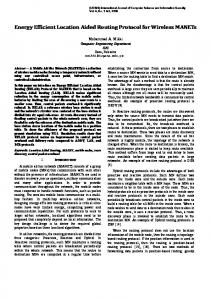
As shown in Figure 2, strategy 1 works well if the correct velocity value is given. The user would reach the next intersection at the time of the next position determination. However, if the user is faster than assumed, she could have left the old location already. In this case, somewhen the location was wrong in the mean time. A slower movement would result in additional position determinations, but not in wrong location assumptions.
Figure 1 visualises an excerpt of the location database, used in our experiments (cf. Section 5). We here focus on street information provided by the OpenStreetMap project (cf. http://www.openstreetmap.org). Hence, our pedestrians’ information system aims to continuously determine the current street the user is located in. The basic idea is that the user has to follow the street until she reaches an intersection (red markers in Figure 1). Hence, knowing the current position, we can calculate the time required for reaching this intersection and delay the next position determination by this time. We used an implementation based on the code of the OpenStreetBlock Web service (cf. http:// frumin.net/ation/2011/04/openstreetblock.html) in order to precalculate intersections.
Static Movement Profiles Our first postponement strategy utilises a pre-defined movement profile, like it is used in most navigation systems. Static profiles assume that the velocity of a movement is almost fixed (based on the types of streets). The used velocity values (e.g. 130 km h−1 on a German autobahn) are experiential average values below the permitted speed lim-
Figure 2: Visualisation of the static strategy.
Adaptive Static Movement Profiles The static movement profile strategy requires more energy if the user is slower than expected and specified in the profile. This might happen if a user stops moving. The authors of [18] introduced a triggering mechanism that analyses the movement by monitoring low-energy sensors, such as the acceleration sensor. Our adaptive static movement profile strategy adapts this idea. The idle time is added to ∆t calculated using Algorithm 1. Monitoring the acceleration sensor obviously requires additional energy. However, as the authors of [9] show, there is a significant difference between the hardware energy requirements. In fact, in our experiments monitoring a non moving device for almost 4 hours required the same amount of energy as 1 GPS-request.
Algorithm 2 Movement monitoring based GPSmeasurement postponement Input: (x, y) ∈ Lname // current position PE (Lname ) // set of location exit points v // velocity value n // trigger interval ss // distance per step 01 def mm wait((x, y), PE (Lname ), v, n, ss ): 02 (∆t, md) = smp wait((x, y), PE (Lname ), v) 03 while (∆t − n > 0) do // we still have to wait 04 sc = count steps(n) // count steps for time n 05 md = md − (ss · sc) // distance still to go 06 v = (ss · sc)/n // update velocity 07 ∆t = md/v // time still to wait 08 done
Personalised, Dynamic Movement Profiles The aforementioned strategies assume that the movement velocity of each pedestrian is either constant or zero. This assumption allows for a quite easy implementation but oversimplifies the reality. Our third strategy takes (in addition to idle times) changes in velocity into account. The basic idea is to update the movement velocity, which is the basis for the GPS-measurement postponement, with each GPSmeasurement. In other words, we personalise the movement profile while walking. Besides GPS polling, one way to measure the real velocity of a pedestrian is to count steps [14] or simply to use “historical” information while assuming that the user moves along a straight path (between two GPSmeasures). Under this assumption we can use the following formalism: Let (xold , yold ) be the last but one measured position, and let told be the point in time of this measurement. Furthermore, let (x, y) be the currently measured position, and let t be the current time. As discussed above, Algorithm 1 suffers from overvaluing the velocity as it leads to too many GPS measurements. However, it does not affect the accuracy of the location determination p negatively. Hence, we use the Euclidean metric sd = (xold − x)2 + (yold − y)2 to calculate the distance between (xold , yold ) and (x, y). As the user needed a time td = t − told for walking this distance, we can simply update the new velocity value to v = sd /td . With this information, the postponement time is calculated using Algorithm 1.
Movement Monitoring Obviously, the best prediction of time of the next required GPS measurement could be done using perfect knowledge about the movement path and the movement velocity. Both could be monitored using GPS polling but this, exactly, is what we want to avoid as we want to reduce the number of GPS requests in order to reduce energy demands. We plan to work on the movement path prediction in future work. Our movement monitoring strategy aims to improve the prediction by adapting ∆t to the current velocity. A proper approach is to count steps by evaluating accelerometer data [14]. Let us assume that a pedestrian covers a distance of ss per step. Let us furthermore assume that md is the minimal distance as defined in Algorithm 1. The idea is to start with an initial velocity v and to update the velocity value every n seconds. Algorithm 2 first calls Algorithm 1 in order to calculate the initial (statically computed) postponement time ∆t and the minimal distance to the closest location exit point md
(line 02). As long as the user would need more time than the predefined step counting interval to leave the location (line 03), the algorithm starts counting the steps for n seconds (line 04). Hence, the algorithm still waits n seconds. Afterwards, it calculates the remaining distance (line 05), the current velocity (line 06), as well as the remaining minimal time to leave the location (line 07) and continues. Please note that Algorithm 2 does not use GPS to update the position while waiting. Hence, it successively decreases ∆t and md even if the user changes the direction of her walking. However, as Algorithm 1 aims to return the minimal time to leave the location Algorithm 2 reduces the problems that would result from a too low static velocity profile value.
5.
EVALUATION
We intentionally decided against conducting a simulation in order to evaluate our algorithms, and conducted a realworld evaluation with Android smartphones instead. This allowed us to gather genuine data about the accuracy, energy demand, and appropriateness of our algorithms. Figure 3 illustrates our test course with the GPS measurement points in red and location exit points in light blue. We will refer back to this visualisation as we discuss the results in more detail.
Setup Our implementation was realised on the Google Android platform as a simple tracking app that logs GPS positions. The app relies on an intersection database that we created using an algorithm for computing road intersections from OpenStreetMap (OSM) data. We adapted the freely available code of the OpenStreetBlock project so that intersection databases for arbitrary regions can be precomputed and stored in SQLite databases. Our modification of the OpenStreetBlock code consists of a python script to scan through the complete OSM data set for a given region (in our case: the city of Weimar and the state of Thuringia), compute all intersections for each street, and build a database of coordinates of intersections. For efficient proximity searches, we used the SpatiaLite (http: //www.gaia-gis.it/gaia-sins/) extension to allow fast indexed perimeter search with R*-trees. A typical query is to select all intersections in the vicinity of a given coordinate and then order them by distance to the given coordinate. The dataset for Weimar includes geographical positions for
(a) SDK
(b) Static
(d) Dynamic
(c) Adaptive
(e) Monitoring
Figure 3: Visualisation of gathered measurements (red markers), location exit points (intersections, light blue markers), and stop points (red dots) on our evaluation course.
2806 intersections, the resulting SQLite database including additional metadata and indexes takes up 4.1 MB on the mobile device. For comparison, the dataset for the state of Thuringia contains 125034 road intersections and takes up 20.3 MB. This illustrates that the required space for the additional data our algorithms need is small enough to include and distribute them with the positioning app. In order to evaluate the number of requests our algorithms generate, the horizontal positioning accuracy of the gathered positions, the energy demands and the location exit hit rate of the algorithms, we used 2 Android devices: an HTC Desire and an HTC Sensation. Both devices are equipped with a high-accuracy GPS chipset, and among a wide range of sensors, an accelerometer. We conducted 9 laps of 1500 m each on an urban course in a low-traffic housing area. Dur-
ing each lap, we were carrying both smartphones and varied the used algorithm. Additionally, we used a dedicated GPS handset (Garmin etrex Legend HCx) to monitor velocity and overall distance. Overall, the average moving velocity was 5.5 km h−1 (4.3 km h−1 including stops), and each lap took about 21 minutes. On each lap, we stopped 2 times for 2 minutes each. The stopping points are highlighted Figure 3. The implementations of the algorithms follow the conceptual description closely: Static assumes a predefined, static velocity to determine the time to wait until the next request is made. Adaptive uses the smartphone’s accelerometer to detect stops and adds this stopping time in the calculation. Dynamic makes also use of this stop trigger and additionally utilises the time and distance between the current and previous request to calculate velocity and then uses this velocity
to compute the wait time. Monitoring finally continuously computes an estimated velocity, based on a step counting mechanism and an assumed stride length.
Number of Requests The first important metric we analysed is the number of GPS requests generated by the algorithms. We assumed that a traditional continuous polling would always generate the most requests, because our proposed algorithms aim to minimise the amount of required requests. In this evaluation, we asked the Android location SDK to send GPS updates with a minimal time interval of 5 seconds, which resulted in 221 requests on the Sensation and 161 on the Desire. This difference results probably in the internal optimisation strategies that trigger additional requests to meet a certain accuracy threshold. regular
static
adaptive
dynamic
monit.
sdk
desire sensation
54 48
38 28
23 30
33 79
161 221
Energy Demand We measured the electrical current and voltage at an interval of 1 Hz using the values generated by the smartphone’s internal power management service. It is not the most exact way to measure power consumption and energy demands, but it enables measurements in the field while actively using the devices (without heavy measurement equipment). energy [kJ]
stat.
adapt.
dyn.
mon.
sdk
idle
desire sensation
0.55 0.58
0.59 0.54
0.53 0.50
0.63 0.92
0.81 0.95
0.33 0.36
0.44 0.40
0.41 0.40
0.44 0.64
0.61 0.72
0.25 0.27
avg. power [watt]
total desire sensation
a lower accuracy per request compared to the SDK method, however our additional accuracy requests successfully address this issue and lower the average accuracy below 15 meters for all algorithms accept number 2, adaptive velocity. This is probably due to the fact that this algorithm has the lowest GPS uptime because it rigorously turns off the chipset when a stop is detected.
132 120
140 151
101 60
57 127
161 221
Table 1: Overview of number of requests across the evaluated algorithms. As Table 1 shows, all algorithms reduce the number of required requests, compared to the SDK baseline. Naturally, the most simple static velocity algorithm requires the most requests because it did not react to the stops we incorporated in our test course and continued to generate requests although the velocity was 0. For each positioning request, we checked the request’s horizontal accuracy and conducted up to 5 additional requests in order to reach a sufficient accuracy below 15 meters. This behaviour mimicks the SDK method’s optimisations.
Horizontal Positioning Accuracy The GPS horizontal positioning accuracy greatly depends on two factors: (1) environmental conditions, such as clear view to the sky or occlusion and reflection by buildings, and (2) the continuous fix time. This second factor describes how long a GPS chipset was continuously switched on and receiving updates. Internal optimisations allow for a greater accuracy compared to selective infrequent GPS requests. This is a great challenge for all algorithms that aim to minimise the continuous uptime of GPS hardware.
desire sensation
0.43 0.45
Table 3: Overview of energy demand and power consumption across the evaluated algorithms. Table 4 shows that the average power consumption and total energy demand is quite stable across our algorithms, with the exception of the monitoring algorithm on the Sensation device. We will discuss the issues of the monitoring algorithm separately at the end of this section. However, it is important to note that even with this outlier, all optimised algorithms perform better than the SDK method. The measured values represent the total energy demand and average power consumption of the entire device. For better comparison, we also measured the devices’ idle baselines. As introduced before, our implementation relies on a local intersection database for location exit point lookups. An alternative approach would be to query the position of the next relevant intersection from a Web service. We implemented a simple web service (in Python) on top of the database and evaluated the difference in power consumption and energy demand for querying the local database versus using the device’s UMTS data connection to query a remote Web service. The results show that the UMTS requests require 32 % more power on average, and 16 % more energy on average. This leaves plenty of room for caching or hoarding strategies to lower this difference.
regular
static
adaptive
dynamic
monit.
sdk
Location Exit Hit Rate
desire sensation
15.04 17.33
20.05 30.46
21.48 16.27
11.61 10.44
7.58 4.50
14.09 14.64
16.20 19.32
14.52 12.90
11.53 11.02
7.58 4.50
The final metric we applied to evaluate our algorithms is a measure for the accuracy of the predicted location exits. Our algorithms aim to minimise the number of unnecessary positioning requests by concentrating on those requests that could be relevant for a location exit. We defined the location exit hit rate as the proportion of number of requests where (1) the street associated with the request (determined by using the reverse geocoder Nomatim) did not change compared to the previous request, (2) the targeted intersection did not change, and (3) the distance to the intersection is greater than the horizontal
total desire sensation
Table 2: Overview of horizontal accuracy across the evaluated algorithms. Table 2 clearly illustrates that all our algorithms result in
static
adaptive
dynamic
monit.
desire sensation
0.94 0.92
0.87 0.86
0.83 0.9
0.94 0.95
avg. distance to exit [meter] desire sensation
23.7 27.4
32.7 35.4
36.7 29.1
32.1 28.0
3
static adaptive
2.5 velocity [m/s]
hit rate
2 1.5 1 0.5
Table 4: Overview of location exit hit rate and average distance to exit points across the evaluated algorithms.
0 0
200
400
600
800
1000
1200
1400
time [s]
(a) Strategies 1 vs. 2 (dotted)
Freedom Degrees Our evaluation results show an obvious difference between theoretic assumptions and real measurements. The reason for this issue is twofold. On the one hand, the algorithms presented in Section 4 are based on perfect knowledge of velocity or step length. On the other hand, real GPS measurements do not return exact positions, but rather approximated ones in combination with an accuracy. The more dynamic parameters a strategy has, the more it suffers from wrong assumptions and imprecise measurements. Figure 4 illustrates real evaluation data of the relationship between time and used or calculated velocity. Obviously, strategy 1 and strategy 2 use a stable velocity. The difference is the handling of stops. However, the only freedom degree is the velocity value defined in the movement profile. The strategies 3 and 4 dynamically adapt the velocity between measurements. Table 1 shows that this does not guarantee a reduction of the number of GPS requests. The reason for this is the increased number of freedom degrees in combination with imperfect measurements. Strategy 3 calculates the new velocity based on the distance between two GPS measures. Remember, GPS measures are circles rather than points. As it is impossible to determine the correct ones, our implementation uses the center points. However, with an accuracy of 15 m, a calculated distance of 100 m corresponds to a range of 70 m . . . 130 m. Hence, we might predict the velocity using the wrong distance value. The more often a strategy adapts the velocity (more peaks in Figure 4), the more often such mistakes might happen. We started experimenting with strategy 4 and varied the
3
dynamic monitoring
2.5 velocity [m/s]
accuracy of the request; divided by the total number of requests. This basically expresses the relation of successful location exit checks to the total number of requests. Requests that are made too early do not lower this rate, but missed intersections do. This expresses the tradeoff between minimising the number of requests and maintaining a required request frequency to recognise location exits. This measure is of course less relevant for the SDK method, because it does not respect location exits and simply polls positions in a predetermined interval. Interestingly, the most simple algorithm 1 (Static) performs best or second-best in this category. The Adaptive and Dynamic algorithms probably reduce the number of requests too far and rely on incorrect assumptions, so that exit points are missed. However, even the lowest hit rate of 83 % is still sufficient in real-world conditions. The best rate of 100 % can probably not even be achieved by the SDK method because of the inaccuracy of the GPS technique and the chosen time interval between requests.
2 1.5 1 0.5 0 0
200
400
600
800
1000
1200
1400
time [s]
(b) Strategies 3 vs. 4 (dotted) Figure 4: Comparison of velocity values among the strategies.
step length. If the velocity is overestimated (we walk slower than expected as we made smaller steps than expected), the system measures too often. If it is underestimated, accuracy decreases. The assumption of 1 m per step, which was an overestimation, resulted in 415 (Desire) and 766 (Sensation) measurements, respectively. The values presented in Table 1 base on a more appropriate step length of 0.55 m.
6.
SUMMARY AND OUTLOOK
In this paper, we addressed the problem of high energy demand for continuous location determination in the context of pedestrian information systems. Even if this domain seems to be extremely specialised, we developed approaches that can be adapted to other movement profiles and domains, as well. We developed, presented, and evaluated four strategies that utilise movement profiles as well as the special extent of locations. The basic idea was to postpone position measurements until location exit points are reached. The evaluation shows that our approaches work well if the required assumptions (velocity, positioning accuracy, distance of steps) are known and accurate. All strategies reduced energy requirements and provided a suitable accuracy. However, they do not consider contextual information. We are planning to analyse accelerometer data in order to learn different pedestrian movement types, such as walking and running, to especially improve strategy 4. The movement type has a direct impact on the step length ss . Furthermore, we plan to evaluate a calibration phase that could personalize velocity values and step length values properly at the beginning of the use of the system.
7.
REFERENCES
[1] C. Becker and F. D¨ urr. On location models for ubiquitous computing. Personal and Ubiquitous Computing, 9(1):20–31, 2005. [2] I. Constandache, S. Gaonkar, M. Sayler, R. R. Choudhury, and L. P. Cox. Energy-Efficient Localization via Personal Mobility Profiling. In T. Phan, R. Montanari, and P. Zerfos, editors, Mobile Computing, Applications, and Services - First International ICST Conference, MobiCASE 2009, San Diego, CA, USA, October 26-29, 2009, Revised Selected Papers, volume 35 of Lecture Notes of the Institute for Computer Sciences, Social Informatics and Telecommunications Engineering (LNICST), pages 203–222, Berlin / Heidelberg, 2010. Springer. [3] Z. Dongqing, L. Zhiping, and Z. Xiguang. Location and its Semantics in Location-Based Services. Geo-spatial Information Science, 10(2):145–150, June 2007. [4] M. Hazas, J. Scott, and J. Krumm. Location-Aware Computing Comes of Age. IEEE Computer, 37(2):95–97, Feb. 2004. [5] I. Heywood, S. Cornelius, and S. Carver. An Introduction to Geographical Information Systems. Prentice Hall, Upper Saddle River, NJ, USA, 2nd edition, Nov. 2002. [6] H. H¨ opfner and C. Bunse. Energy Awareness Needs a Rethinking in Software Development. In M. J. Escalona, B. Shishkov, and J. Cordeiro, editors, Proceedings of the 6th International Conference on Software and Data Technologies, ICSOFT 2011, Seville, Spain, July 18-21, 2011, volume 2, pages 294–297, Set´ ubal, Portugal, July 2011. INSTICC, SciTePress. ISBN: 978-989-8425-77-5. [7] E. Hornecker, S. Swindells, and M. Dunlop. A mobile guide for serendipidous exploration of cities. In Proceedings of the 13th International Conference on Human Computer Interaction with Mobile Devices and Services – MobileHCI’11, pages 557–562, New York, NY, USA, 2011. ACM. [8] M. Kenteris, D. Gavalas, and D. Economou. An innovative mobile electronic tourist guide application. Personal and Ubiquitous Computing, 13(2):103–118, February 2009. [9] M. B. Kjærgaard, J. Langdal, T. Godsk, and T. Toftkjær. EnTracked: energy-efficient robust position tracking for mobile devices. In MobiSys’09 Proceedings of the 7th international conference on Mobile systems, applications, and services, Wroclaw, Poland, June 22-25, 200, pages 221–234, New York, NY, USA, 2009. ACM Press. [10] R. L. Knoblauch, M. T. Pietrucha, and M. Nitzburg. Field Studies of Pedestrian Walking Speed and Start-Up Time. Transportation Research Record: Journal of the Transportation Research Board, 1538:27–38, 1996. [11] K. Lin, A. Kansal, D. Lymberopoulos, and F. Zhao. Energy-accuracy trade-off for continuous mobile device location. In Proceedings of the 8th international conference on Mobile systems, applications, and services, San Francisco, CA, USA, June 15-18, 2010, pages 285–297, New York, NY, USA, 2010. ACM.
[12] Y. Ma, R. Hankins, and D. Racz. iloc: a framework for incremental location-state acquisition and prediction based on mobile sensors. In Proceedings of the 18th ACM Conference on Information and Knowledge Management – CIKM’09, pages 1367–1376, New York, NY, USA, 2009. ACM. [13] E. Miluzzo. Smartphone Sensing. PhD thesis, Darttmouth College, Hanover, NH, USA, June 2011. available online http://sensorlab.cs.dartmouth. edu/pubs/miluzzo-phd-dissertation.pdf. [14] M. Mladenov and M. Mock. A step counter service for java-enabled devices using a built-in accelerometer. In Proceedings of the 1st International Workshop on Context-Aware Middleware and Services: affiliated with the 4th International Conference on Communication System Software and Middleware – COMSWARE 2009, pages 1–5, New York, NY, USA, 2009. ACM. [15] B. Pernici, editor. Mobile Information Systems — Infrastructure and Design for Adaptivity and Flexibility. Springer, Berlin, 2006. [16] B. Priyantha, D. Lymberopoulos, and J. Liu. Little rock: Enabling energy-efficient continuous sensing on mobile phones. IEEE Pervasive Computing, 10(2):12–15, Apr.-June 2011. [17] S. Robinson, M. Jones, P. Eslambolchilar, R. Murray-Smith, and M. Lindborg. ”i did it my way”: Mobving away from the tyranny of turn-by-turn pedestrian navigation. In Proceedings of the 12th International Conference on Human Computer Interaction with Mobile Devices and Services – MobileHCI’10, pages 341–344, New York, NY, USA, 2010. ACM. [18] M. Schirmer and H. H¨ opfner. SenST: Approaches for Reducing the Energy Consumption of Smartphone-Based Context Recognition. In M. Beigl, H. Christiansen, T. Roth-Berghofer, A. Kofod-Petersen, K. R. Coventry, and H. R. Schmidtke, editors, Proceedings of the 7th International and Interdisciplinary Conference on Modeling and Using Context 2011 (CONTEXT’11); September 26-30, 2011, Karlsruhe, Germany, volume 6967 of Lecture Notes in Computer Science, pages 250–263, Berlin / Heidelberg, 2011. Springer. ISBN: 978-3-642-24278-6. [19] A. Y. Seydim, M. H. Dunham, and V. Kumar. Location dependent query processing. In S. Banerjee, editor, Proceedings of the 2nd ACM international workshop on Data engineering for wireless and mobile access, Santa Barbara, CA, USA, May 20, 2001, pages 47–53, New York, NY, USA, 2001. ACM. [20] J. Ye, L. Coyle, S. Dobson, and P. Nixon. A unified semantics space model. In J. Hightower, B. Schiele, and T. Strang, editors, Proceedings of the 3rd International Symposium on Location- and Context-Awareness (LoCA 2007), September 20-21, 2007, Oberpfaffenhofen, Germany, LNCS, pages 103–120, Berlin/Heidelberg, 2007. Springer. [21] P. A. Zandbergen. Accuracy of iPhone Locations: A Comparison of Assisted GPS, WiFi and Cellular Positioning. Transactions in GIS, 13(s1):5–26, July 2009.