Department of Electrical Engineering. University of California, Los Angeles ... that the optimum total transmit power (water level) depends not only on the MIMO ...
Energy-efficient power loading for a MIMO-SVD system and its performance in flat fading Raghavendra S. Prabhu, Babak Daneshrad Department of Electrical Engineering University of California, Los Angeles Email: {ragh, babak}@ee.ucla.edu Abstract—In this paper we formulate a power loading problem for the spatial subchannels (parallel channels) of a single-carrier MIMO-SVD system. The power loading solution is designed to minimize the energy-per-goodbit (EPG) of the MIMO-SVD system. The optimum power loading obtained by solving a nonlinear fractional program, has a closed-form expression and is found by applying a water-filling procedure. It is observed that the optimum total transmit power (water level) depends not only on the MIMO channel realization, but also on the ratio of circuit power cost (which depends on the number of antennas) to transmit power cost (which depends on path loss and other factors). We study the statistical performance (using simulation) of the solution in Rayleigh and Rician flat-fading channels. Using outage EPG as a measure of performance, we determine the MIMO configuration (from a set of allowed configurations) that yields the minimum outage EPG. It is observed that the average number of spatial subchannels utilized (which indicates preference for diversity or multiplexing) depends on the ratio of circuit power cost to transmit power cost and fading type (Rayleigh or Rician). For both cases, the results show that both multiplexing and diversity obtained by MIMO systems are critical for energy efficiency.
I. I NTRODUCTION It is well known that systems with multiple antennas at transmitter and receiver, generally referred to as multipleinput multiple-output (MIMO) systems, can provide dramatic improvements in spectral efficiency [1] and reliability [2], without requiring any additional bandwidth or transmit power. However, using multiple radio chains incurs a higher circuit power consumption. Assuming perfect channel state information (CSI) at both the transmitter and receiver, a MIMOSVD architecture uses the singular value decomposition (SVD) beamforming to effectively create parallel independent channels in space. These spatial subchannels typically possess different levels of quality or signal-to-noise ratio (SNR). Transmit power is an important resource, which effectively determines the rate, reliability and energy consumption of the system. Desired system performance can then be optimized by carefully allocating power at the transmitter to each subchannel depending on its quality. Depending on the operating conditions, it may be more energy efficient to limit the transmission to a few of the best quality subchannels (using one subchannel results in maximal diversity [2]) or it may be better to utilize all subchannels to achieve a high rate (multiplexing). In this paper, we find the power allocation that maximizes energy efficiency and then study the trade off between the diversity
and/or mutliplexing of multiple antennas and the higher circuit power consumption by focusing on energy efficiency of the wireless link. Related work in the MIMO power loading literature has been focused on optimizing either rate, total transmit power, bit error rate, etc. [3], [4]. In this paper we are interested in maximizing energy efficiency (equivalently minimizing EPG). Recently adaptive modulation has been used to provide substantial gains in energy efficiency especially in cases where the energy consumed by communication circuitry is not negligible [5], [6]. This work has also been extended to a MIMO scenario [7], where space-time block codes (STBC) are used to provide diversity. In contrast to [7], we assume perfect CSI at the transmitter and hence limit our focus to the MIMO-SVD scheme. In [8] an energy-efficient water-filling algorithm was developed for a single antenna orthogonal frequency division multiplexing (OFDM) system, where it was shown that the transmit power water level must be carefully chosen for energy-efficient operation. The work in this paper is an extension of the work in [8] to MIMO systems, where the parallel channels are in space. Note that the energy model here is different from [8], since there is now a cost for every additional degree of freedom (circuit power for each transmit and receive antenna pair). In this paper we also characterize the energy-efficient MIMO configurations under Rayleigh and Rician fading for different transmit costs. Although the solution and algorithms presented here are easily extended to frequency-selective MIMO-OFDM systems, we will restrict our attention to the quasistatic flatfading scenario, which is in some sense a worst-case scenario where spatial diversity is the only form of diversity available. The outline of the paper is as follows. The problem is formulated in section II, after describing the system model and the objective function. In section III, the solution and an algorithm to obtain the optimal power allocation is described. In section III, we define and discuss statistical measures of performance. In section IV, we present the results obtained from conducting a statistical performance analysis with the help of a numerical (simulation) example. In section V, the paper is concluded. II. P ROBLEM FORMULATION A. System preliminaries We consider a point-to-point wireless single-carrier nT ×nR MIMO-SVD system with Nss spatial subchannels, where nT
and nR are the number of transmit and receive antennas respectively. Bits from a packet of length L bits are coded and modulated, where coded bits are mapped to a constellation symbol xi at an average power GPi for each subchannel i ∈ {1, 2, . . . , Nss }, where we define G as the constant transmit power that is needed to overcome deleterious effects such as path loss, implementation loss and thermal noise, but also takes into account the benefits of coding gain (or equivalently SNR gap) and antenna gain. The constant transmit power G is defined as � �−2 λ G = ML Γ(BER) d κ No Nf B , (1) 4π where ML is the link margin to account for implementation imperfections in the system, λ is the wavelength at the carrier frequency, d is the distance between the transmitter and receiver and κ is the path-loss exponent. We also scale G by the variance of the additive thermal noise observed at the receiver. This noise is modeled as additive white Gaussian noise (AWGN) with variance σ 2 = No Nf B, where No /2 is the two-sided noise power spectral density (PSD), Nf is the the noise figure of the receiver and B is the bandwidth of the system. Assuming a fixed operating bit error rate (BER), BER, we can compute the SNR gap approximation Γ(BER) for a given coded modulation scheme [9]. As a simple example, an approximate SNR gap (from Shannon limit) for uncoded −1 ) . Similar to [10], we assume QAM is Γ(BER) = log(BER 1.5 a packet based system with ARQ in a long-term static fading channel. B. Signal model The received signal y ∈ CnR is a linear transformation of transmit signal s ∈ CnT plus an additive noise w ∈ CnR , y = Hs + w, where H ∈ CnR ×nT is the MIMO channel matrix and w has i.i.d. complex Gaussian elements with zero-mean and unit variance. The SVD factorization of H, which always exists, is given as H = UΣV† , where U is a nR × nR unitary matrix whose columns are the eigenvectors of the matrix HH† , V is a nT × nT unitary matrix whose columns are the eigenvectors of the matrix H† H and Σ is a nR × nT diagonal matrix, whose diagonal elements are nonnegative p real numbers called singular values and are given by [Σ]i,i = λi (HH† ) for i = 1, 2, . . . , r, where λi (HH† ) or simply λi is the i-th largest eigenvalue of matrix HH† and r denotes the rank of H. Note that [Σ]i,i = 0 for i = r + 1, . . . , min(nT , nR ). The signals sent over transmit antennas s are obtained by performing a linear transformation s = VPx, where by a slight abuse of notation, V is a nT × Nss transmit beamforming/precoding matrix obtained from the SVD of H, P is a Nss × Nss diagonal matrix where [P]i,i = Pi for i = 1, 2, . . . , Nss , where Pi is the transmit power allocated to the i-th spatial subchannel and x ∈ ANss is the information symbol vector drawn from unit-energy constellation set A. Since the power allocation Pi determines whether the i-th
spatial subchannel is used or not, we may assume Nss = min(nT , nR ) without any loss in generality. In the MIMO-SVD scheme, the received signal y is linearly processed by a Nss × nR matrix, U† , obtained from the SVD of H to yield y ˜ = U† y = ΣPx + w, ˜ (2) p √ √ where Σ = diag( λ1 , λ2 , . . . , λNss ) (slight abuse of notation) and w ˜ = U† w is an equivalent noise vector with i.i.d. complex Gaussian elements with zero-mean and unit variance. The signal model in (2) is a parallel channel model where the effective receiver signal to noise ratio (SNR) for subchannel i is γi Pi , where γi is the receiver (sub)channel to noise ratio (CNR) of subchannel i and is defined as γi = σλ2i , where σi2 i is the variance of the noise and interference experienced by subchannel i. If there is no interference and only thermal noise, then the normalization of G implies that effectively σi2 = 1. The bits per symbol or spectral efficiency of subchannel i is given by bi = log2 (1 + γi Pi ). The (or bits per vector PNrate ss log2 (1 + γi Pi ). symbol), R, is expressed as R = i=1 C. Objective function: energy-per-goodbit (EPG)
The objective function that corresponds to EPG may be derived by following similar steps and assumptions found in [11], [10]. We express EPG as a function of the vector variable P = [P1 , P2 , . . . , PNss ], which corresponds to transmit power without the constant scale factor G. The EPG for a singlecarrier MIMO-SVD system is then defined as PNss Pi + NA kc kt , (3) Ea (P) = PNss i=1 i=1 log2 (1 + γi Pi )
where kt and kc are non-negative constants which are interpreted as transmit and circuit EPG respectively for unit αG transmit power and unit rate, and are given by kt = (1−PER)B Pc and kc = (1−PER)B , respectively. Parameters in the model include, α = OBO ηmax , where OBO is the output backoff from saturation power level of the power amplifier (PA) and ηmax is the maximum PA efficiency (or drain efficiency), PER is the packet error rate (PER), Pc is the average power consumption in a single transmit or receiver chain (the rest of the transmit and receive electronics excluding the PA). For a MIMO system, Pc is computed as Pc =
nT Pc,tx + nR Pc,rx + Pco , NA
(4)
where Pc,tx and Pc,rx are the power consumed in a single transmit chain and receive chain, Pco is the (common) power consumed independent of the number of antennas and the total number of antennas in the system, NA = nT + nR . D. Energy minimization problem For a given nT × nR MIMO configuration and channel realization, H, the MIMO-SVD scheme results in a CNR vector γ. The goal is then to find the power allocation, P∗ , that results in the minimum EPG, Ea (P∗ ), subject to certain constraints, such as a minimum rate constraint (Rmin ), a total
transmit power constraint (PT ) and Pmax is an upper bound on the maximum allowed power per subchannel (this is the same as a per-antenna power constraint if we take into account the PA backoff). The optimization problem can be stated as: minimize Ea (P) PNss subject to i=1 Pi ≤ PT 0 ≤ Pi ≤ Pmax , i = 1, 2, . . . , Nss PNss i=1 log2 (1 + γi Pi ) ≥ Rmin
(5)
It is clear that the constraints above are convex. However, it is not clear that the objective function Ea (P) is convex, but it may be classified as a nonlinear fractional programming problem. III. S OLUTION AND PERFORMANCE MEASURE A. Optimum power allocation The power allocation derived in [8] which was shown to be the globally optimum solution to an objective function essentially the same as given in (3) can be directly applied (with some minor changes) to obtain the optimum power allocation P∗ . We only present the brief steps needed to obtain the solution and refer the reader to [8] for details. It can be shown that the optimum power allocation for subchannel i for a given parameter q which will be found later, has the following form: �P � 1 max q + ν∗ q − , (6) Pi = ln(2)(kt + λ∗ ) γi 0 where λ∗ is the optimal dual variable corresponding to the total power constraint and ν ∗ is the optimal dual variable corresponding to the minimum rate constraint. It can be observed that parameter q controls the water level. The parameter q will be obtained by solving a nonlinear equation and modified (if necessary) by applying one or more water-filling procedures. B. Water-filling algorithm In this section we enumerate a sequence of steps that arrive at the optimal energy-efficient power allocation. ∗ Step 1: Find unconstrained EPG qUC The optimum power allocation without minimum rate and total power constraints is obtained by setting dual variables ∗ ν ∗ and λ∗ in (6) to zero. Then qUC is the solution to the following nonlinear equation: �P Nss � X 1 max q − + NA µd f (q) = ln(2)kt γi 0 i=1 � �P ! Nss X q 1 max log2 1 + γi −q − = 0, ln(2)kt γi 0 i=1
where µd is defined as the ratio of circuit to transmit EPG for unit rate and power, i.e. µd = kkct . We note that a solution always exists for this problem [8]. For an increasing circuit power consumption (represented by increasing NA µd ), we can deduce that q (water level) needs to increase and vice-versa.
Step 2: Apply rate constraint � � minimum PNss q∗ log2 1 + γi Pi UC > Rmin , then by complementary If i=1 slackness, ν ∗ = 0. Otherwise, ν ∗ is the solution to �P ! � ∗ Nss X 1 max qUC + ν ∗ − = Rmin (7) log2 1 + γi ln(2)kt γi 0 i=1 In this case the minimum EPG is achieved by the maximize margin power allocation [12]. For easy reference, we define ∗ ∗ qMM = qUC + ν ∗ , so that the power allocation after applying ∗ qMM step 2 is P .
Step 3: Apply total power constraint ∗ PNss qMM P < PT , then by complementary slackness, If i=1 i λ∗ = 0. Otherwise there are two possibilities: 1) The problem is infeasible if ν ∗ > 0. This can be thought of as an outage event. 2) If ν ∗ = 0, λ∗ is the solution to �P Nss � ∗ X 1 max qUC − = PT (8) ln(2)(kt + λ∗ ) γi 0 i=1 With the above modified power allocation, we need to check again if the minimum rate constraint is violated and if so the problem is infeasible. If there is no outage, then the minimum EPG is achieved by the classical rate maximization power allocation. C. Outage EPG as performance measure In the previous subsection we saw that the optimum power allocation and consequently the minimum EPG that results, is a function of the MIMO channel via the CNR vector γ. When the MIMO fading channel matrix follows a probability distribution, there may be a set of channel matrices that are very poor in quality or cost too much EPG. In these cases, it may make sense to turn off the radio completely (outage event). Service requirements dictate the maximum tolerated outage probability, po . A percentile measure is the value of a variable below which a certain percent of observations fall. Thus a (1 − po ) × 100% percentile EPG or equivalently po × 100% outage EPG is the highest cost (in EPG) that a user will incur in order to communicate a bit. In a similar manner, outage spectral efficiency gives the slowest rate at which a user will communicate. Outage transmit power gives the maximum power that will be used. Although closed-form expressions for ordered eigenvalues of Wishart matrices are available, the complicated (nonlinear) nature of the water-filling procedure makes it difficult to analyze performance without resorting to simulation. As a result, we characterize the statistical variation of the minimum EPG and optimum power allocation using simulation. In the next section, various antenna configurations will be compared in terms of the outage EPG. IV. N UMERICAL EXAMPLE The parameters (unless specified otherwise) used in the numerical example are given in table I. We assume that wave8 length is calculated as λ = 3×10 fc . We compute PER using the
TABLE I PARAMETER VALUES USED IN NUMERICAL EXAMPLE Parameter Name
Symbol
Value
Packet length System bandwidth Path-loss exponent Carrier frequency Noise PSD Noise figure Circuit power Output backoff Max. PA efficiency Link margin Operating BER Gap (Uncoded QAM) Outage probability level
L B κ fc N0 /2 Nf Pc OBO ηmax Ml BER Γ(BER) po
2000 bits 100 kHz 3.5 2.4 GHz −204 dBW/Hz 10 dB 200 mW 10 dB 0.35 10 dB 10−5 8.9 dB 0.05
L
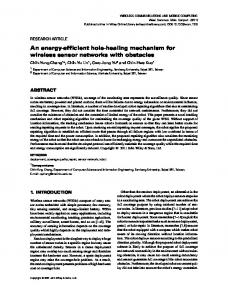
formula PER = 1 − (1 − BER) , which is an approximation. A realization of the CNR vector γ is generated by finding the eigenvalues of the Wishart matrix H† H (assuming nR > nT ). Each (i, j)-th element in a MIMO channel matrix realization is an i.i.d. random variable with the following distribution r r K 1 [H]i,j ∼ + CN (0, 1) , K +1 K +1 where K is called the Rician K-factor and is the power (strength) of the constant line-of-sight (LOS) component relative to the random non-LOS component. The results are obtained by simulating 80,000 independent channel realizations for each MIMO configuration. For purposes of clarity, we are not imposing any minimum rate, total transmit power or peak power constraint (although these constraints are easily handled, see section III). Moreover, the outage formulation already gives an indication of minimum rate and maximum total transmit power. A. Most energy-efficient MIMO configuration The most energy-efficient MIMO configuration or optimum MIMO configuration, nT,EE × nR,EE ∈ NMIMO , is defined to be the MIMO configuration that yields the smallest outage EPG (at a specific po ). The optimum configuration is chosen from a discrete and (in practice) finite set of allowed MIMO configurations NMIMO . We consider balanced MIMO configurations limited to a maximum of four antennas at either end. For a given total number of antennas, balanced MIMO configurations provide superior capacity. Since we have assumed symmetric circuit energy costs at both transmitter and receiver, an X × Y configuration is equivalent to a Y × X configuration. It should be noted that the equivalence will generally not hold when there is spatial correlation. In our case, the search space can be reduced by removing equivalent configurations. Thus the set of allowed MIMO configurations are NMIMO = {1 × 1, 1 × 2, 2 × 2, 2 × 3, 3 × 3, 3 × 4, 4 × 4}. Notice that the number of antennas, NA = nT + nR uniquely determines the configuration. If NA∗ denotes the optimum
or most energy-efficient number of antennas, then nT,EE × nR,EE = ⌊NA∗ /2⌋×⌈NA∗ /2⌉. The number of subchannels used for a given channel realization is the cardinality of the power allocation vector, which depends on the channel realization and µd . For a specified value of µd , the average number of subchannels used, with an abuse of notation, Nss , gives an indication of the preference for multiplexing and/or diversity. Figure 1 shows the optimum MIMO configuration at a 5% outage level (po = 0.05) over a range of µd , over Rayleigh (K = 0) and Rician (K = 10) fading. For Rayleigh fading, the largest MIMO configuration is always preferred irrespective of the transmit cost or circuit cost. The mean subchannel utilization Nss indicates that high multiplexing is preferred when circuit cost is high and diversity is preferred as transmit cost increases. This makes sense since the water level is high when µd is large and low when µd is small. When there is a relatively significant LOS component (K = 10), MIMO configurations are preferred for their diversity benefits when transmit costs are dominant or relatively comparable (µd < 102 ). When circuit costs dominate (µd > 102 ), Rician channels do not provide sufficient multiplexing that allows a higher rate and as a result a single-input singleoutput (SISO) configuration is optimum. Peculiarly there is a region, when circuit costs are comparable to transmit costs (10−1 < µd < 102 ), where having multiple radio chains is not so costly and also the water level is high enough to support some amount of spatial multiplexing. Figures 2, 3 and 4 show the outage EPG, the outage rate and the outage total transmit power respectively, for the optimum MIMO configuration NA∗ and for a SISO configuration NA = 2, for both Rayleigh and Rician fading. From Fig. 2, it can be seen that MIMO configuration outperforms the SISO configuration over the whole range of µd for the Rayleigh fading case. In the case of Rician fading, the benefits of MIMO come into play when transmit costs become comparable to circuit costs. MIMO provides significant increase in outage rate under Rayleigh fading (Fig. 3). For the Rayleigh fading case and when circuit cost dominate (µd > 2), we observe that the outage total transmit power (Fig. 4) for the optimum MIMO configuration is higher than that for the corresponding SISO case. This is because the higher power is used to provide high rate (multiplexing gain). When transmit costs dominate, MIMO provides a more reliable channel (diversity) which allows a much lower transmit power compared to SISO (for both fading cases) to maintain the outage level. V. C ONCLUSION We obtained a power loading solution that minimized the energy-per-goodbit (EPG) of a MIMO-SVD system. Using a numerical example, we found the most energy-efficient MIMO configuration for both Rayleigh and Rician flat-fading channels, using outage EPG as the performance metric. From the results we can conclude that both multiplexing (more so for Rayleigh fading) and diversity of MIMO systems are critical for energy-efficient operation. Practical considerations such as
40
4 35
NA∗ , K = 0 NA = 2, K = 0 NA∗ , K = 10 NA = 2, K = 10
3.5 30
K = 0, NA∗ /2 K = 0, mean Nss
Outage rate (b/s/Hz)
NA∗ /2 and Nss
3
K = 10, NA∗ /2 K = 10, mean Nss
2.5
2
25
20
15
10
1.5 5
1 −2
0
10
10
2
µd
4
10
0 −4 10
6
10
10
Fig. 1. Most energy-efficient MIMO configuration and spatial subchannel utilization. The x-axis is µd = kkc , the ratio of circuit and transmit EPG for t unit total power and rate. Results shown for both Rayleigh (K = 0, blue) and Rician (K = 10, red) fading. 30
−1
10
0
10
1
µd
10
kc , kt
2
10
3
4
10
10
5
10
the ratio of circuit and transmit
40
NA∗ , K = 0 NA = 2, K = 0 NA∗ , K = 10 NA = 2, K = 10
35
Outage transmit power (dBm)
30
10 Outage EPG (dBmJ)
−2
10
Fig. 3. Outage rate. The x-axis is µd = EPG for unit total power and rate.
NA∗ , K = 0 NA = 2, K = 0 NA∗ , K = 10 NA = 2, K = 10
20
−3
10
0
−10
25
20
15
10 −20
5 −30
0 −4 10 −40 −4 10
−2
10
0
10
2
4
10
10
µd
Fig. 2. Outage EPG. The x-axis is µd = EPG for unit total power and rate.
kc , kt
6
10
−2
10
0
10
2
10
µd
4
10
6
10
8
10
8
10
Fig. 4. Outage total transmit power. The x-axis is µd = circuit and transmit EPG for unit total power and rate.
kc , kt
the ratio of
the ratio of circuit and transmit
impact of channel estimation error and channel feedback costs on energy efficiency are areas of further research. R EFERENCES [1] E. Telatar, “Capacity of multi-antenna Gaussian channels,” European trans. on telecommunications, vol. 10, no. 8, pp. 585–595, 1999. [2] P. Dighe, R. Mallik, and S. Jamuar, “Analysis of transmit-receive diversity in Rayleigh fading,” IEEE Trans. Commun., vol. 51, no. 4, pp. 694–703, Apr. 2003. [3] Z. Zhou, B. Vucetic, M. Dohler, and Y. Li, “MIMO systems with adaptive modulation,” IEEE Trans. Veh. Technol., vol. 54, no. 5, pp. 1828–1842, Sept. 2005. [4] A. Lozano, A. M. Tulino, and S. Verdu, “Optimum power allocation for parallel Gaussian channels with arbitrary input distributions,” IEEE Trans. Inf. Theory, vol. 52, no. 7, pp. 3033–3051, Jul. 2006. [5] C. Schurgers, O. Aberthorne, and M. Srivastava, “Modulation scaling for energy aware communication systems,” in International Symposium on Low Power Electronics and Design, Aug. 2001, pp. 96–99.
[6] S. Cui, A. Goldsmith, and A. Bahai, “Energy-constrained modulation optimization,” IEEE Trans. Wireless Commun., vol. 4, no. 5, pp. 2349– 2360, Sept. 2005. [7] ——, “Energy-efficiency of MIMO and cooperative MIMO techniques in sensor networks,” IEEE J. Sel. Areas Commun., vol. 22, no. 6, pp. 1089–1098, Aug. 2004. [8] R. S. Prabhu and B. Daneshrad, “An energy-efficient water-filling algorithm for OFDM systems,” in IEEE International Conference on Communications, May 2010. [9] J. Forney, G.D. and G. Ungerboeck, “Modulation and coding for linear Gaussian channels,” IEEE Trans. Inf. Theory, vol. 44, no. 6, pp. 2384– 2415, Oct. 1998. [10] R. Prabhu and B. Daneshrad, “Energy minimization of a QAM system with fading,” IEEE Trans. Wireless Commun., vol. 7, no. 12, pp. 4837– 4842, Dec. 2008. [11] R. Prabhu, B. Daneshrad, and L. Vandenberghe, “Energy minimization of a QAM system,” in IEEE Wireless Communications and Networking Conference, Mar. 2007, pp. 729–734. [12] N. Papandreou and T. Antonakopoulos, “Bit and power allocation in constrained multicarrier systems: the single-user case,” EURASIP Journal on Advances in Signal Processing, vol. 2008, no. 1, 2008.