Energy-Efficient SPEED Routing Protocol for Wireless Sensor ...

2009 Fifth Advanced International Conference on Telecommunications

Energy-efficient SPEED Routing Protocol for Wireless Sensor Networks Mohammad Sadegh Kordafshari, Azadeh Pourkabirian -

Department of Computer Engineering and IT Qazvin Azad University, QIAU Qazvin, Iran e-mail:{ kordafshari, pourkabirian}@qazviniau.ac.ir

Karim Faez

Ali Movaghar Rahimabadi

Department of Electrical Engineering Department of Computer Engineering Amirkabir University of technology Sharif University of technology Tehran, Iran Tehran, Iran e-mail: [email protected] e-mail: [email protected]

\\\

Abstract— In this paper, we propose an approach for routing in SPEED protocol considering residual energy in routing decisions. Due to the limited energy of a sensor node, energyefficient routing is a very important issue in sensor networks. This approach finds energy-efficient paths for delayconstrained data in real-time traffic. The SPEED protocol does not consider any energy metric in its routing. In our approach, routing is based on a weight function, which is a combination of the three factors: Delay, Energy & Speed. Here, the node with the greatest value in the weight function is to be selected as the next hop forwarding. We increase the network lifetime by considering energy metric in routing decisions. This method aims to construct a nearly stateless routing protocol, which can be used to route data based on the nodes’ residual energy. Simulation results demonstrate that the new scheme improves network lifetime about 15% longer than the traditional SPEED protocol.

Energy-efficient SPEED routing protocol (EE-SPEED) that balances energy consumption. Our approach takes the energy factor within routing decisions into consideration, preventing the exclusive selection of special nodes for routing. Therefore, we prevent from discharge of energy on special nodes and increase network lifetime. The three basic factors are Delay, Energy and Speed for routing decisions. Simulation results demonstrate that the new scheme improves network lifetime more than the traditional SPEED protocol. The rest of this paper is organized as follows: Section II gives a brief description of the SPEED protocol, and lists the drawbacks of the previous works. The proposed EE-SPEED protocol is depicted in Section III. In Section IV, four performance metrics are defined and the results from a comprehensive experiment are presented and analyzed. Finally, section V, comes up with a brief conclusion.

Keywords: Sensor Network; SPEED protocol; energy efficient; QoS routing

II. RELATED WORK

.

Recently, wireless sensor networks have spread and are used for different uses [5]. One of the most common one is the real time applications and services, where the quality of service parameter is considered, after which the quality of service routing protocols [6] are invented. Now we briefly survey some of the previous works in the field. There are many approaches to QoS routing in sensor networks; but most of them do not consider energy consumption during the communication. RAP [7] uses velocity monotonic scheduling to prioritize real-time traffic and to enforce such prioritization through a differentiated MAC Layer. The other protocol for sensor networks that includes the notion of QoS in its routing decisions is the Sequential Assignment Routing (SAR) [8]. The SAR protocol creates trees routed from one-hop neighbor of the sink by taking QoS metric, energy resource on each path and priority level of each packet into consideration. By using the created trees, multiple paths from sink to the sensors are formed. Consequently, one of the paths can be selected according to the energy resources and QoS on each path. In addition, the SAR approach suffers from the overhead of maintaining the node states at each sensor node. SPEED [3] is a routing protocol that provides soft end-to-end delay guarantees for sensory data transfers. While SPEED takes into account the delay caused by channel access mechanisms, it pays no attention to the energy expended along the selected path. In

I. INTRODUCTION A sensor network [1] consists of a large number of smart sensing devices, referred as sensor nodes. They have a limited energy supply, for which routing protocols must be low-power. Here, a new approach for routing in SPEED protocol is suggested. The SPEED protocol is a quality of service routing protocol that guarantees end-to-end delay for real-time traffic. Routing decisions in this protocol are based on a single hop delay and relay speed. This protocol considers no energy metric on its routing. Hence, energy depletion of selected nodes will be faster [3]. One way to reach energy efficiency is the use of greedy geographical routing [2] which SPEED protocol [3] utilizes to make localized routing decisions. Greedy geographic-based routing [4] tends to reduce the number of hops in the route. It always takes the local shortest path, resulting in reducing the energy consumed in transmissions. However, there is a problem of energy depletion of sensors on shortest paths; so the network is being partitioned in nearly a short time. In order to solve this problem, the energy consumption in all the nodes should be balanced. We present a scheme called

978-0-7695-3611-8/09 $25.00 © 2009 IEEE DOI 10.1109/AICT.2009.52

267

Authorized licensed use limited to: QUEENSLAND UNIVERSITY OF TECHNOLOGY. Downloaded on July 4, 2009 at 07:46 from IEEE Xplore. Restrictions apply.

view of this, the key design goal of the SPEED algorithm is to support a soft real-time communication service with a desired delivery speed across the sensor network, so that end-to-end delay is proportional to the distance between the source and destination. Our work is inspired by SPEED [3].

and the neighbor node with highest relay speed has a higher probability to be chosen as the forwarding node. Relay speed is calculated by dividing the advance in distance from the next hop node j by the estimated delay to forward a packet to node j. Formally, Relayspeed = (|L – L_next | / SingleHopDelay)

III. SPEED PROTOCOL OVERVIEW

IV.

Our solutions are emanated by SPEED [14]. Similar to other geographic routing algorithms, every node in SPEED periodically broadcasts a beacon packet to its neighbors. This periodic beaconing is only used for exchanging information ( NeighborID, Position, SingleHopDelay, ExpireTime) between neighbors. Every node has a neighbor table, which consists of a list of all its neighbors, where there is an entry for each neighbor. The ExpireTime is used to timeout this entry in a neighbor table. The algorithm uses single hop delay as the metric to approximate the load of a node. Delay is measured at the sender, which timestamps the packet entering the network output queue and calculates the round trip single hop delay for this packet when receiving the ACK. At the receiver side, the duration for processing an ACK is put into the ACK packet. Propagation delay is ignored. Every node has a Neighbor Set which is the set of nodes that are inside the radio range R of node i. Formally, NSi= {node | distance (node, node i) ≤ R}

(3)

ENERGY EFFICIENT ROUTING

A. Assumption Consider a network of n sensor nodes with none replenish able energy which are randomly placed in a network. We assume that the initial energy distribution on nodes is imbalanced, for the energy depletion rate is not the same on various nodes in the network. Some nodes have to expend more energy due to their location in the network. For example, nodes closer to the base station are in a critical region, because they have to forward data continuously, which results in draining their energies much faster than the other nodes. Our key design goal of this algorithm is to optimize energy consumption in the nodes, as we wish to prevent energy depletion on special nodes by balancing the load on them. By this technique we avoid partitioning of the network and increase its lifetime. Network lifetime can be defined as the time it takes for the first node or a fraction of nodes in the network to be depleted of their energies. Since the lower energy nodes are what the network lifetime depends on, it becomes necessary to offer them more protection. The main advantage of our approach to SPEED protocol is protecting the nodes with less energy to avoid their discharge and to have the nodes with more energy. First step in our algorithm is to get the residual energy of the nodes. Next, we will form a weight function by which we could perform routing.

(1)

A set of nodes that belong to NSi(K) and are at least K distance closer to the destination than a current node i are forming the Forwarding Candidate Set of Node i. Formally,

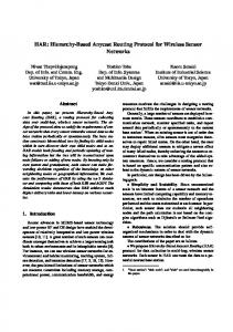
FS i ( Destination) = {node ∈ NS i L − L _ next > k} (2) Where L is the distance from node i to the destination and L_next is the distance from the next hop candidate node to the destination (Figure1).

B. Energy model We suppose that there is an unbalanced distribution of initial energy on the nodes. Therefore, the sink node and the neighboring ones have more initial energy than the others. We show the residual energy on node j by Ej, calculated based on the following formula [9]:

Ej =

E 0 − CE j E0

(4)

Where E0 is the initial energy and CEj is the consumed energy of node j, which can be calculated based on the model in [10]. Energy consumption of each sensor is simply defined as the normalized total amount of energy spent in receiving or sending messages, i.e., CEj. Therefore, for each node, by having E0 value and calculating CEj, as in [10], we could calculate its residue energy. As we had in SPEED protocol [3], every node periodically broadcasts a beacon packet to its neighbors. The information passed by

Figure 1. NS & FS Definition

SPEED divides the neighbor nodes inside FSi(Destination) into two groups. One consists of nodes having a SingleHopDelay less than the certain single hop delay D. The other includes nodes having a SingleHopDelay longer than the certain single hop delay D. The forwarding candidate is chosen from the first group,

268


the beaconing is stored in a neighboring table. Each entry inside the table has the following fields: (NeighborID, Position, SingleHopDelay, ExpireTime, and Residual Energy). Every node is location-aware [11]. Then, all nodes inside NSi set send their information to node i, and it saves them in FSi set, which uses this information to select the next hop for its routing.

forwarding based on the results. Our protocol routes the packets according to the following rules: 1. First, for each node, the neighbor set (NSi) is formed according to [3]. 2. By beacon exchanging, each node gains the required information of the neighbors inside its NSi set and maintains them in its FSi set. 3. According to this information, the value of the weight function is calculated for all nodes in the FSi set. 4. Among the nodes belonging to the FSi set, the node with highest value in weight function will be chosen as the next hop forwarding candidate, to which the packet is sent. Using this algorithm, end to end delay is supported for a packet, like [3]; In addition, by considering the energy metric in the routing decisions, we can prevent energy depletion of special nodes (the nodes that have the highest speed, as well as the previous delay condition).

C. Weight Function Definition and Calculation The current node i, considers its FSi set as the forwarding candidate. The forwarding candidate is chosen from this set, and the neighbor node with the highest value in the weight function has a higher probability to be chosen as the forwarding node. This weight function is formally defined as [9]:

f = max(α .En + β .Sp ∗ φ ( De))

α + β =1

Where

and V. EXPERIMENTATION AND EVALUATION

⎧1 → De > 1 ϕ ( De) = ⎨ ⎩ z → De < 1

(5)

Here, we simulate our approaches on C++ and compare them with SPEED routing protocol. Different parameters are considered: 1) end-to-end delay under different congestion levels, 2) The number of control packets, 3) network lifetime and energy consumption. The experiment was conducted in two network areas of 80 × 80m2 and 500 × 500m2, for a network size of 10, 40, 65 and 80. Each sensor has an initial energy of 1J; and base station was located in (25, 145) and (500, 700), respectively. Each sensor node generates a fixed length packet size of 1000 bits. All nodes are placed randomly in the specific network field. Each experiment is repeated 14 times with different random seeds and different random node topologies.

Here, fj is the weight function value of the jth sensor; En is the ratio of residual energy on node j, De is the ratio of delay on node j, and Sp is the relay speed its packet transfers from the present node to node j. α and β are the coefficients of these factors. Having any of them reduced to zero, the corresponding component will no more be considered. Now, we define each factor separately. So the residual energy is calculated as [12]:

En j =

Ej E max

(6)

Where Ej is the value of residual energy on node j, and Emax is the highest value of residual energy on nodes in FSi set. The ratio of delay is:

De j =

D dj

A. End-to-End Delay Delay is one important metric for the real time traffic, which always must be considered. SPEED protocol guarantees end-to-end delay for the real time traffic. As shown in Figure1, EE-SPEED protocol has a longer delay than SPEED; but end-to-end delay is supported for packets in this algorithm, because, like before, the delay threshold is considered in making routing decisions. It’s possible that the node chosen as the next hop forwarding candidate has the most residual energy and its delay is more than the others. Although the delay of this node is slightly greater than that of the others, this node does not have any disallowed delay; besides, the aim of this algorithm is to increase network lifetime. Consequently, the node is chosen as the next hop forwarding candidate. Sometimes the delay in this algorithm exceeds that of the SPEED protocol, but as the simulation results indicate, this is never more than the delay threshold and thereby will support end-

(7)

Where D is the possible maximum delay in a single hop, (same as the delay threshold) and dj is the delay value on node j (singlehopdelay). The last parameter is calculated based on the following formula [3]:

Sp j =

l − l _ next Singlehopdelay

(8)

Where l is the distance from node i to the destination, l_next is the distance from the next hop forwarding candidate node to the destination, and delay is the estimated delay to forward a packet to node j. Now, by calculating all parameters of the weight function for all neighbors inside NSi related to node i, we can calculate the weight function for each of these neighbors, and select the next hop of

269


to-end delay. This increase of delay can be ignored due to the network’s longer lifetime. Delay Threshold (D)

0.8

0.7

End-to-end Delay

0.6

0.5

0.4

0.3

0.2

Figure4. Residual energy of nodes

SPEED EB-SPEED

0.1

Suppose that the energy consumed in node i for each sending/receiving to/from a node as j is eij; we can calculate the energy consumed at node i according to the passed flows from this node in various times of simulation. rij is the rate of information flow from the node i to the node j. Consequently the lifetime of the node i can be estimated as follows [13]: Error! Objects cannot be created from editing field codes. (9) Where, Ei is the initial energy of node i. Therefore, we can define the network lifetime as the time it takes for the first node in the network to be depleted of its energies. It is formulated as follows: Error! Objects cannot be created from editing field codes. (10) Our purpose is to maximize Ti for the nodes to increase the network lifetime.

0 0

5

10

15

20

Number of Flow

25

Figure2. End-to-end delay under different congestion

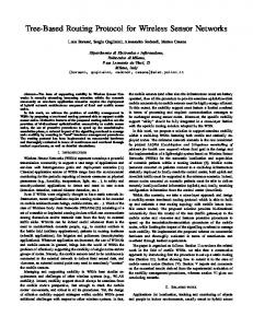
B. Number of control packets The control packets used in our algorithm, are the beacons that are sent to the neighbors immediately after energy changing of the nodes to inform these changes. These packets update the information inside the NS set of each nodes’ neighbors. In the SPEED protocol, if we have 100 nodes, simulated for 14 times in conditions stated in [3], the average of these control packets will be between 900 and 1050. In our method, at the worst case, this number is 1200 (Figure 2). This occurs when the sending/receiving rate in nodes is high, since the energy is discharged by each sending/receiving, by which a beacon is to be sent to the neighbors to recognize the nodes' residual energy. In this algorithm, we periodically ignore the sending beacons and consider them as on-demand. N um ber of C ontrol Packets

1600

1400

1200

1000

800

600

400

EB_SPEED SPEED

200

0 0

1

3

5

7

9

11

13

15

17

19

Number of Flows

Figure5. Average network lifetime

Figure3. Number of control packet

The different streams tend to select minimum-hop paths on which nodes die sooner and therefore, limit the network lifetime. The simulation results show a definite improvement in terms of energy distribution and the average time it takes for the low nodes in the network to die. We compare the network lifetime of protocols which is the time taken for 1/3rd of all the nodes to die and protocols have shown similar values in the initial stages of the network.

C. Network Lifetime Note that, as is evident in figures 3 and 4, one of the disadvantages of SPEED protocol is that it does not consider the metric of energy in routing decisions. In this case, the energy will be depleted in special nodes which will cause the network to be partitioned. The proposed algorithm in this paper prevents this problem by considering the energy metric, which itself will increase the network lifetime.

D. Energy Consumption In the SPEED protocol, delay and relay speed are two important parameters in routing decisions. The nodes on special paths that have the least delay and the most relay

270


speed die sooner than the others. Figure 5 shows the energy consumption on these nodes. As it shows, in the specific time of simulation, the special nodes’ energy depleted sooner than the others and it caused the network to be partitioned. EE-SPEED protocol tries to make the nodes’ residual energy balanced, which causes better energy consumption on nodes. As demonstrated in Figure 5, by balancing the energy consumption on nodes, the network will be partitioned later and the network can be used longer.

REFERENCES [1] [2] [3]

[4]

[5] [6] [7]

[8] [9]

[10] [11] [12] Figure6. Energy usage in EE-SPEED and SPEED

VI. CONCLUSION In this paper, we proposed an algorithm for routing in the SPEED protocol that concentrates on energy-efficient routing. In this algorithm, the idea is to combine the cost and metric the quality of service metric on nodes to select the path by considering the three parameters of Delay, Energy and Speed. Simulation results and a comparison of this algorithm with the SPEED protocol represent that distributing energy consumption on nodes in routing will protect the nodes with less energy and prevents from a fast destruction. This, directly, causes the network lifetime to increase. However, a problem should be considered in the SPEED protocol, furthermore: How can we guarantee the successful delivery of the data packets in such a randomly distributed sensor network? For instance, in an extreme case where the sink node happens to be a set in an isolated place, how can we deliver the data packets?

[13]

F. Akyildiz, W. Su, Y, Sankarasubramaniam, and E. Cayirci, “A Survey on Sensor Networks,” IEEE Communications, Aug. 2003, pp. 102-114. B. Karp and H. T. Kung. “GPSR: Greedy Perimeter Stateless Routing for Wireless Networks,”. In IEEE MobiCom, August 2004. T. He, J. Stankovic, C. Lu, and T. Abdelzaher, “SPEED: A Stateless Protocol for Real-Time Communication in Sensor Networks,” Proceedings of IEEE International Conference on Distributed Computing Systems, pp. 46–55, 2005. Y. Xu, J. Heidemann, and D. Estrin. “Geography-informed Energy Conservation for Ad Hoc Routing,” In Proceedings of the Seventh Annual ACM/IEEE International Conference on Mobile Computing and Networking (MobiCom 2003), Rome Italy, July 16-21, 2003. A. Mainwaring et al., “Wireless sensor networks for habitat monitoring,”Proceedings of the ACM WSNA, Atlanta, GA, September 2004. T. Chen, J. Tsai, and M. Gerla, “QoS Routing Performance in Multihop Multimedia Wireless Networks,” Proc. IEEE Sixth Int’l Conf. Universal Personal Comm., vol. 2, pp 557-561, 2003. C. Lu, B. Blum, T. Abdelzaher, J. Stankovic, and T. He.” RAP: A Real- Time Communication Architecture for Large-Scale Wireless Sensor Networks,” In IEEE Real-time Applications Symposium, 2002. K. Sohrabi, J. Gao, V. Ailawadhi, and G. J. Potie, "Protocols for selforganization of a wireless sensor network,” IEEE Personal Communications, pp. 16-27, October 2005. K.i. Sha, J. Du, and W. Shi ”WEAR: A Balanced, FaultTolerant, Energy-Aware Routing Protocol for Wireless Sensor Networks,” International Journal of Sensor Networks (IJSNet), Vol. 1, No. 2, 2006. K. Sha and W. Shi. “Modeling the lifetime of wireless sensor networks,”. Technical Report MIST-TR-2004-011, Wayne State University, Oct. 2004. Y.B. Ko and N. H. Vaidya. “Location-Aided Routing(LAR) in Mobile Ad Hoc Networks,”. In IEEE MobiCom 2000, October 2000. L.Gan, J. Liu, and X. Jin,” Agent-Based, Energy Efficient Routing in Sensor Networks,” International Conference on Autonomous Agents Proceedings of the Third International Joint Conference on Autonomous Agents and Multiagent Systems, New York , Vol. 1, pp 472 - 479 , 2004. T. He et al., “Energy-Efficient Surveillance Systems Using Wireless Sensor Networks,” Proceeding of the ACM MobiSys, 2004.

271
