the prelude that describes the code. We present experimental results that com- pare our new method with previous approaches to byte coding, in terms of both.
Enhanced byte codes with restricted prefix properties J. Shane Culpepper1 and Alistair Moffat2 1. NICTA Victoria Laboratory, Department of Computer Science and Software Engineering, The University of Melbourne, Victoria 3010, Australia 2.
Department of Computer Science and Software Engineering The University of Melbourne, Victoria 3010, Australia
Abstract. Byte codes have a number of properties that make them attractive for practical compression systems: they are relatively easy to construct; they decode quickly; and they can be searched using standard byte-aligned string matching techniques. In this paper we describe a new type of byte code in which the first byte of each codeword completely specifies the number of bytes that comprise the suffix of the codeword. Our mechanism gives more flexible coding than previous constrained byte codes, and hence better compression. The structure of the code also suggests a heuristic approximation that allows savings to be made in the prelude that describes the code. We present experimental results that compare our new method with previous approaches to byte coding, in terms of both compression effectiveness and decoding throughput speeds.
1 Introduction While most compression systems are designed to emit a stream of bits that represent the input message, it is also possible to use bytes as the basic output unit. For example, Scholer et al. [2002] describe the application of standard byte codes – called vbyte encoding in their paper – to inverted file compression; and de Moura et al. [2000] consider their use in a compression system based around a word-based model of text. In this paper we describe a new type of byte code in which the first byte of each codeword completely specifies the number of bytes that comprise the suffix of the codeword. The new structure provides a compromise between the rigidity of the static byte codes employed by Scholer et al., and the full power of a radix-256 Huffman code of the kind considered by de Moura et al. The structure of the code also suggests a heuristic approximation that allows savings to be made in the prelude that describes the code. Rather than specify the codeword length of every symbol that appears in the message, we partition the alphabet into two sets – the symbols that it is worth taking care with, and a second set of symbols that are treated in a more generic manner. Our presentation includes experimental results that compare the new methods with previous approaches to byte coding, in terms of both compression effectiveness and decoding throughput speeds.
2 Byte-aligned codes In the basic byte coding method, denoted in this paper as bc, a stream of integers x ≥ 0 is converted into a uniquely decodeable stream of bytes as follows: for each integer
x, if x < 128, then x is coded as itself in a single byte; otherwise, (x div 128) − 1 is recursively coded, and then x mod 128 is appended as a single byte. Each output byte contains seven data bits. To force the code to be prefix-free, the last output byte of every codeword is tagged with a leading zero bit, and the non-final bytes are tagged with a leading one bit. The following examples show the simple byte code in action – bytes with a decimal value greater than 127 are continuers and are always followed by another byte; bytes with a decimal value less than 128 are stoppers and are terminal. 0 → 000 1 → 001 2 → 002
1,000 → 134-104 1,001 → 134-105 1,002 → 134-106
1,000,000 → 188-131-064 1,000,001 → 188-131-065 1,000,002 → 188-131-066
To decode, a radix-128 value is constructed. For example, 188-131-066 is decoded as ((188 − 127) × 128 + (131 − 127)) × 128 + 66 = 1,000,002. The exact origins of the basic method are unclear, but it has been in use in applications for more than a decade, including both research and commercial text retrieval systems to represent the document identifiers in inverted indexes. One great advantage of it is that each codeword finishes with a byte in which the top (most significant) bit is zero. This identifies it as the last byte before the start of a new codeword, and means that compressed sequences can be searched using standard pattern matching algorithms. For example, if the three-element source sequence “2; 1,001; 1,000,000” is required, a bytewise scan for the pattern 002-134-105-188-131-064 in the compressed representation will find all locations at which the source pattern occurs, without any possibility of false matches caused by codeword misalignments. In the terminology of Brisaboa et al. [2003b], the code is “end tagged”, since the last byte of each codeword is distinguished. de Moura et al. [2000] consider byte codes that are not naturally end-tagged. The simple byte code is most naturally coupled to applications in which the symbol probabilities are non-increasing, and in which there are no gaps in the alphabet caused by symbols that do not occur in the message. In situations where the distribution is not monotonic, it is appropriate to introduce an alphabet mapping that permutes the sparse or non-ordered symbol ordering into a ranked equivalent, in which all mapped symbols appear in the message (or message block, if the message is handled as a sequence of fixed-length blocks), and each symbol is represented by its rank. Brisaboa et al. [2003b] refer to this mapping process as generating a dense code. For example, consider the set of symbol frequencies: 20, 0, 1, 8, 11, 1, 0, 5, 1, 0, 0, 1, 2, 1, 2 that might have arisen from the analysis of a message block containing 53 symbols over the alphabet 0 . . . 14. The corresponding dense frequency distribution over the alphabet 0 . . . 10 is generated by the alphabet mapping [0, 4, 3, 7, 12, 14, 2, 5, 8, 11, 13] → [0, 1, 2, 3, 4, 5, 6, 7, 8, 9, 10] , that both extracts the n = 11 subset of alphabet symbols that occur in the message, and also indicates their rank in the sorted frequency list. Using dense codes, Brisaboa et al. were able to obtain improved compression when the underlying frequency distribution was not monotonically decreasing, with compressed searching still possible by mapping the pattern’s symbols in the same manner. Our experimentation below includes a
permuted alphabet dense byte coder, denoted dbc. The only difference between it and bc is that each message block must have a prelude attached to it, describing the alphabet mapping in use in that block. Section 4 considers in more detail the implications of including a prelude in each block of the compressed message. In followup work, Brisaboa et al. [2003a] (see also Rautio et al. [2002]) observe that there is nothing sacred about the splitting point of 128 used to separate the stoppers and the continuers in the simple byte coder, and suggest that using values S and C, with S + C = 256, gives a more flexible code, at the very small cost of a single additional parameter in the prelude. One way of looking at this revised scheme is that the tag bit that identifies each byte is being arithmetically coded, so that a little more of each byte is available for actual “data” bits. The codewords generated by a (S, C)-dense coder retain the end-tagged property, and are still directly searchable using standard character-based pattern matching algorithms. The same per-block prelude requirements as for the dbc implementation apply to scdbc, our implementation of (S, C)-dense coding. Brisaboa et al. describe several mechanisms for determining an appropriate value of S (and hence C) for a given frequency distribution, of which the simplest is brute-force – simply evaluating the cost of each alternative S, and choosing the S that yields the least overall cost. Pre-calculating an array of cumulative frequencies for the mapped alphabet allows the cost of any proposed set of codeword lengths to be evaluated quickly, without further looping. Brute-force techniques based on a cumulative array of frequencies also play a role in the new mechanism described in Section 3. Finally in this section, we note that Brisaboa et al. [2005] have recently described an adaptive variant of the (S, C)-dense mechanism, in which the prelude is avoided and explicit “rearrange alphabet mapping now” codes are sent as needed.
3 Restricted prefix byte codes The (S, C)-dense code is a byte-level version of the Golomb code [Golomb, 1966], in that it matches best with the type of self-similar frequency sets that arise with a geometric probability distribution. For example, once a particular value of S has been chosen, the fraction of the available code-space used for one byte codewords is S/(S + C); of the code-space allocated to multi-byte codewords, the fraction used for two byte codes is S/(S + C); and so on, always in the same ratio. On the other hand, a byte-level Huffman code of the kind examined by de Moura et al. [2000] exactly matches the probability distribution, and is minimum-redundancy over all byte codes. At face value, the Huffman code is much more versatile, and can assign any codeword length to any symbol. In reality, however, a byte-level Huffman code on any plausible probability distribution and input message block uses just four different codeword lengths: one byte, two bytes, three bytes, and four bytes. On an nsymbol decreasing probability distribution, this observation implies that the set of dense symbol identifiers 0 . . . (n−1) can be broken into four contiguous subsets – the symbols that are assigned one-byte codes, those given two-byte codes, those given three-byte codes, and those given four-byte codes. If the sizes of the sets are given by h1 , h2 , h3 , and h4 respectively, then for all practical purposes a tuple (h1 , h2 , h3 , h4 ) completely defines a dense-alphabet byte-level Huffman code, with n = h1 + h2 + h3 + h4 .
0
1
20
2
11
3
8
4
5
v1=2 00
01 00
5
2
6
2
7
1
8
1
9
1
10
1
21
1
v2=1
v3=1
10 prefix followed by
11 prefix followed by
01
10
11
00 00
00 01
00 10
00 11
01 00
.....
11 11
Fig. 1. Example of a restricted prefix code with R = 4 and n = 11, and (v1 , v2 , v3 ) = (2, 1, 1). The codewords for symbols 11 to 21 inclusive are unused. The 53 symbols are coded into 160 bits, compared to 144 bits if a bitwise Huffman code is calculated, and 148 bits per symbol if a radix-4 Huffman code is calculated. Prelude costs are additional.
In the (S, C)-dense code, the equivalent tuple is infinite, (S, CS, C 2 S, . . .), and it is impossible, for example, for there to be more of the total codespace allocated to twobyte codewords than to one-byte codewords. On a input message that consists primarily of low probability symbols, compression effectiveness must suffer. Our proposal here adds more flexibility. Like the radix-256 Huffman code, we categorize an arrangement using a 4-tuple of numbers (v1 , v2 , v3 , v4 ), and require that the Kraft inequality be satisfied. But the numbers in the tuple now refer to initial digit ranges in the radix-R code, and are set so that v1 + v2 + v3 + v4 ≤ R. The code itself has v1 one-byte codewords; Rv2 two-byte codewords; R2 v3 three-byte codewords; and R3 v4 four-byte ones. To be feasible, we thus also require v1 +v2 R+v3 R2 +v4 R3 ≥ n, where R is the radix, typically 256. We will denote as restricted prefix a code that meets these criteria. The codeword lengths are not as freely variable as in an unrestricted radix-256 Huffman code, but the loss in compression effectiveness compared to a Huffman code is slight. Figure 1 shows an example code that has the restricted prefix property, calculated with a radix R = 4 for a dense alphabet covering n = 11 symbols. In this code, the first two-bit unit in each codeword uniquely identifies the number of two-bit units in the suffix. Two symbols have codes that are one unit long (v1 = 2); four symbols have codes that are two units long, prefixed by 10; and five symbols have codes that are two units long, prefixed by 11. There are eleven unused codewords. The great benefit of the additional constraint is that the first unit (byte) in each codeword unambiguously identifies the length of that codeword, in the same way that in the K-flat code of Liddell and Moffat [2004] each codeword commences with a k-bit binary prefix that determines the length of the suffix part for that codeword, for some fixed value k. In particular, for the code described by (v1 , v2 , v3 , v4 ), the first byte of any one-byte codeword will be in the range 0 . . . (v1 − 1); the first byte of any two-byte codeword in the range v1 . . . (v1 + v2 − 1); and the first byte of any three-byte codeword will lie between (v1 + v2 ) . . . (v1 + v2 + v3 − 1). With this structure, it is possible to create an R-element array suffix that is indexed by the first byte of each codeword and exactly indicates the total length of that codeword. Algorithm 1 shows how the suffix array, and a second array called first, are initialized, and then used during the decoding process. Once the codeword length is known,
Algorithm 1 : Decoding a message block. input: a block-length m, a radix R (typically 256), and control parameters v1 , v2 , v3 , and v4 , with v1 + v2 + v3 + v4 ≤ R. 1: create tables(v1 , v2 , v3 , v4 , R) 2: for i ← 0 to m − 1 do 3: assign b ← get byte() and offset ← 0 4: for i ← 1 to suffix [b] do 5: assign offset ← offset × R + get byte() 6: assign output block [i] ← first [b] + offset output: the m symbols coded into the message block are available in the array output block function create tables(v1 , v2 , v3 , v4 , R) 1: assign start ← 0 2: for i ← 0 to v1 − 1 do 3: assign suffix [i] ← 0 and first [i] ← start and start 4: for i ← v1 to v1 + v2 − 1 do 5: assign suffix [i] ← 1 and first [i] ← start and start 6: for i ← v1 + v2 to v1 + v2 + v3 − 1 do 7: assign suffix [i] ← 2 and first [i] ← start and start 8: for i ← v1 + v2 + v3 to v1 + v2 + v3 − v4 − 1 do 9: assign suffix [i] ← 3 and first [i] ← start and start
← start + 1 ← start + R ← start + R2 ← start + R3
Algorithm 2 : Seeking forward a specified number of codewords. input: the tables created by the function create tables (), and a seek offset s. 1: for i ← 0 to s − 1 do 2: assign b ← get byte() 3: adjust the input file pointer forwards by suffix [b] bytes output: a total of s − 1 codewords have been skipped over.
the mapped symbol identifier is easily computed by concatenating suffix bytes together, and adding a pre-computed value from the first array. The new code is not end tagged in the way the (S, C)-dense method is, a change that opens up the possibility of false matches caused by byte misalignments during pattern matching. Algorithm 2 shows the process that is used to seek forward a fixed number of symbols in the compressed byte stream and avoid that possibility. Because the suffix length of each codeword is specified by the first byte, it is only necessary to touch one byte per codeword to step forward a given number s of symbols. By building this mechanism into a pattern matching system, fast compressed searching is possible, since standard pattern matching techniques make use of “shift” mechanisms, whereby a pattern is stepped along the string by a specified number of symbols. We have explored several methods for determining a minimum-cost reduced prefix code. Dynamic programming mechanisms, like those described by Liddell and Moffat [2004] for the K-flat binary case, can be used, and have asymptotically low execution costs. On the other hand, the space requirement is non-trivial, and in this preliminary study we have instead made use of a generate-and-test approach, described in Algorithm 3, that evaluates each viable combination of (v1 , v2 , v3 , v4 ), and chooses the one with the least cost. Even when n > 105 , Algorithm 3 executes in just a few hundredths
Algorithm 3 : Calculating the code split points using a brute force approach. input: a set of n frequencies, f [0 . . . (n − 1)], and a radix R, with n ≤ R4 . 1: assign C[0] ← 0 2: for i ← 0 to n − 1 do 3: assign C[i + 1] ← C[i] + f [i] 4: assign mincost ← partial sum(0, n) × 4 5: for i1 ← 0 to R do 6: for i2 ← 0 to R − i1 do 7: for i3 ← 0 to R − i1 − i2 do 8: assign i4 ← d(n − i1 − i2 R − i3 R2 )/R3 e 9: if i1 + i2 + i3 + i4 ≤ R and cost (i1 , i2 , i3 , i4 ) < mincost then 10: assign (v1 , v2 , v3 , v4 ) ← (i1 , i2 , i3 , i4 ) and mincost ← cost (i1 , i2 , i3 , i4 ) 11: if i1 + i2 R + i3 R2 ≥ n then 12: break 13: if i1 + i2 R ≥ n then 14: break 15: if i1 ≥ n then 16: break output: the four partition sizes v1 , v2 , v3 , and v4 . function partial sum(lo, hi): 1: if lo > n then 2: assign lo ← n 3: if hi > n then 4: assign hi ← n 5: return C[hi] − C[lo] function cost (i1 , i2 , i3 , i4 ) 1: return partial sum(0, i1 ) × 1 + partial sum(i1 , i1 + i2 R) × 2 + partial sum(i1 + i2 R, i1 + i2 R + i3 R2 ) × 3 + partial sum(i1 + i2 R + i3 R2 , i1 + i2 R + i3 R2 + i4 R3 ) × 4
or tenths of a second, and requires no additional space. In particular, once the cumulative frequency array C has been constructed, on average just a few hundred thousand combinations of (i1 , i2 , i3 , i4 ) are evaluated at step 9, and there is little practical gain in efficiency possible through the use of a more principled approach.
4 Handling the prelude One of the great attractions of the simple bc byte coding regime is that it is completely static, with no parameters. To encode a message, nothing more is required than to transmit the first message symbol, then the second, and so on through to the last. In this sense it is completely on-line, and no input buffering is necessary. On the other hand, all of the dense codes are off-line mechanisms – they require that the input message be buffered into message blocks before any processing can be started. They also require that a prelude be transmitted to the decoder prior to any of the codewords in that block.
As well as a small number of scalar values (the size of the block; and the code parameters v1 , v2 , v3 , and v4 in our case) the prelude needs to describe an ordering of the codewords. For concreteness, suppose that a message block contains m symbols in total; that there are n distinct symbols in the block; and that the largest symbol identifier in the block is nmax . The obvious way of coding the prelude is to transmit a permutation of the alphabet [Brisaboa et al., 2003a,b]. Each of the n symbol identifiers requires approximately log nmax bits, so to transmit the decreasing-frequency permutation requires a total of n log nmax bits, or an overhead of (n log nmax )/m bits per message symbol. When n and nmax are small, and m is large, the extra cost is negligible. For character-level coding applications, for example with n ≈ 100 and nmax ≈ 256, the overhead is less than 0.001 bits per symbol on a block of m = 220 symbols. But in more general applications, the cost can be non-trivial. When n ≈ 105 and nmax ≈ 106 , the overhead cost on the same-sized message block is 1.9 bits per symbol. In fact, an exact permutation of the alphabet is not required – all that is needed is to know, for each alphabet symbol, whether or not it appears in this message block, and how many bytes there are in its codeword. This realization leads to a better way of describing the prelude: first of all, indicate which n-element subset of the symbols 0 . . . nmax appears in the message block; and then, for each symbol that appears, indicate its codeword length. For example, one obvious tactic is to use a bit-vector of nmax bits, with a zero in the kth position indicating “k does not appear in this message block”, and a one in the kth position indicating that it does. That bit-vector is then followed by a set of n two-bit values indicating codeword lengths between 1 and 4 bytes. Using the values n ≈ 105 and nmax ≈ 106 bits, the space required would thus be nmax + 2n ≈ 1.2 × 10⁶, or 1.14 bits per symbol overhead on a message block of m = 220 symbols. Another way in which an ordered subset of the natural numbers can be efficiently represented is as a sequence of gaps, taking differences between consecutive items in the set. Coding a bit-vector is tantamount to using a unary code for the gaps, and more principled codes can give better compression when the alphabet density differs significantly from one half, either globally, or in locally homogeneous sections. In a byte coder, where the emphasis is on easily decodeable data streams, it is natural to use a simple byte code for the gaps. The sets of gaps for the symbols with one-byte codes can be encoded; then the set of gaps of all symbols with two-byte codes; and so on. To estimate the cost of this prelude arrangement, we suppose that all but a small minority of the gaps between consecutive symbols are less than 127, the largest value that is coded in a single byte. This is a plausible assumption unless, for example, the sub-alphabet density drops below around 5%. Using this arrangement, the prelude costs approximately 8n bits, and when n ≈ 105 corresponds to 0.76 bit per symbol overhead on a message block of m = 220 symbols. The challenge is to further reduce this cost. One obvious possibility is to use a code based on half-byte nibbles rather than bytes, so as to halve the minimum cost of coding each gap. But there is also another way of improving compression effectiveness, and that is to be precise only about high-frequency symbols, and to let low-frequency ones be assigned default codewords without their needing to be specified in the prelude. The motivation for this approach is that spending prelude space on rare symbols may, in the long run, be more expensive than simply letting them be represented with their “natural” sparse codes.
Algorithm 4 : Determining the code structure with a semi-dense prelude. input: an integer nmax , and an unsorted array of symbol frequency counts, with c[s] recording the frequency of s in the message block, 0 ≤ s ≤ nmax ; together with a threshold t. 1: assign n ← 0 2: for s ← 0 to nmax do 3: assign f [t + s].sym ← s and f [t + s].freq ← c[s] 4: identify the t largest freq components in f [t . . . (t + nmax )], and copy them and their corresponding symbol numbers into f [0 . . . (t − 1)] 5: for s ← 0 to t − 1 do 6: assign f [f [s].sym ].freq ← 0 7: assign shift ← 0 8: while f [t + shift] = 0 do 9: assign shift ← shift + 1 10: for s ← t + shift to nmax do 11: assign f [s − shift] ← f [s] 12: use Algorithm 3 to compute v1 , v2 , v3 , and v4 using the t + nmax + 1 − shift elements now in f [i].freq 13: sort array f [0 . . . (t − 1)] into increasing order of the sym component, keeping track of the corresponding codeword lengths as elements are exchanged 14: transmit v1 , v2 , v3 , and v4 and the first t values f [0 . . . (t − 1)].sym as a prelude, together with the matching codeword lengths for those t symbols 15: sort array f [0 . . . (t − 1)] into increasing order of codeword length, with ties broken using the sym component 16: for each symbol s in the message block do 17: if ∃x < t : f [x].sym = s then 18: code s as the integer x, using v1 , v2 , v3 , and v4 19: else 20: code s as the integer t + s − shift, using v1 , v2 , v3 , and v4
Algorithm 4 gives details of this semi-dense method, and Figure 2 gives an example. A threshold t is used to determine the number of high-frequency symbols for which prelude information is supplied in a dense part to the code; and all symbols (including those in the dense code) are allocated sparse codewords. A minimum-redundancy restricted prefix code for the augmented symbol set is calculated as before; because the highest frequency symbols are in the dense set, and allocated the shortest codewords, compression effectiveness can be traded against prelude size by adjusting the control knob represented by t. For example, t might be set to a fixed value such as 1,000, or might be varied so as to ensure that the symbols that would originally be assigned one-byte and two-byte codewords are all in the dense set. Chen et al. [2003] describe a related mechanism in which symbols over a sparse alphabet are coded as binary offsets within a bucket, and a Huffman code is used to specify bucket identifiers, based on the aggregate frequency of the symbols in the bucket. In their method, each bucket code is sparse and self-describing, and the primary code is a dense one over buckets. In contrast, we partially permute the alphabet to create a dense region of “interesting” symbols, and leave the uninteresting ones in a sparse zone of the alphabet.
0
1
2
3
4
5
6
7
8
9
10
11
12
13
14
20
0
1
8
11
1
0
5
1
0
0
1
2
1
2
20
11
8
5
(0)
0
1
(0)
(0)
1
0
(0)
1
0
0
1
2
20
11
8
5
1
(0)
(0)
1
0
(0)
1
0
0
1
2
1
2
11 00
11 01
1
2
11 10
11 11
t=4 v1=3 00
01
v3=1 11 prefix followed by
10 00 00
00 01
00 10
00 11
01 00
.....
Fig. 2. Example of a semi-dense restricted prefix code with R = 4, nmax = 14, and a threshold of t = 4. The largest four frequencies are extracted, and the rest of the frequency array shifted right by four positions, with zeros inserted where elements have been extracted. In the third row, shift = 2 leading zeros are suppressed. The end array has t + nmax + 1 − shift = 13 elements, and is minimally represented as a (v1 , v2 , v3 ) = (3, 0, 1) code, with a cost of 162 bits. The modified prelude contains only four symbols, seven less than is required when the code is dense.
5 Experiments Table 1 describes the four test files used to validate the new approach to byte coding. They are all derived from the same source, a 267 MB file of SGML-tagged newspaper text, but processed in different ways to generate streams of integer symbol identifiers. The first two files are of particular interest, and can be regarded as respectively representing the index of a mid-sized document retrieval system, and the original text of it. In this example the index is stored as a sequence of d-gaps (see Witten et al. [1999] for a description of inverted index structures), and the text using a word-based model. Table 2 shows the compression effectiveness achieved by the experimental methods for the four test files described in Table 1, when processed as a sequence of message blocks (except at the end of the file) of m = 220 symbols. Table 2 does not include any prelude costs, and hence only those for the basic byte coder bc represent actual achievable compression. The file wsj267.repair shows the marked improvement possible with the rpbc approach compared to the scdbc method – on this file there are almost no one-byte codewords required, and a large number of two-byte codewords. The first three columns of Table 3 show the additional cost of representing a dense prelude, again when using blocks of m = 220 symbols. Storing a complete permutation of the alphabet is never effective, and not an approach that can be recommended. Use of a bit-vector is appropriate when the sub-alphabet density is high, but as expected, the gap-based approach is more economical when the sub-alphabet density is low. The fourth column of Table 3 shows the cost of the semi-dense prelude approach described in Section 4. It is expressed in two parts – the cost of a partial prelude de-
wsj267.ind: Inverted index d-gaps
Total Maximum n/nmax Self-information symbols value (m = 220 ) (bits/sym) 41,389,467 173,252 10.4% 6.76
wsj267.seq: Word-parsed sequence
58,421,983 222,577
22.5%
10.58
wsj267.seq.bwt.mtf: Word-parsed sequence BWT’ed and MTF’ed
58,421,996 222,578
20.8%
7.61
wsj267.repair: Phrase numbers from 19,254,349 320,016 a recursive byte-pair parser
75.3%
17.63
File name and origin
Table 1. Parameters of the test files. The column headed “n/nmax ” shows the average subalphabet density when the message is broken into blocks each containing m = 220 symbols.
File wsj267.ind wsj267.seq wsj267.seq.bwt.mtf wsj267.repair
Method bc 9.35 16.29 10.37 22.97
dbc 9.28 12.13 10.32 19.91
scdbc 9.00 11.88 10.17 19.90
rpbc 8.99 11.76 10.09 18.27
Table 2. Average codeword length for different byte coding methods. Each input file is processed as a sequence of message blocks of m = 220 symbols, except at the end. Values listed are in terms of bits per source symbol, excluding any necessary prelude components. Only the column headed bc represents attainable compression, since it is the only one that does not require a prelude.
scribing the dense subset of the alphabet, plus a value that indicates the extent to which compression effectiveness of the rpbc method is reduced because the code is no longer dense. In these experiments, in each message block the threshold t was set to the sum v1 + v2 R generated by a preliminary fully-dense evaluation of Algorithm 3, so that all symbols that would have been assigned one-byte and two-byte codes were protected into the prelude, and symbols with longer codes were left in the sparse section. Overall compression is the sum of the message cost and the prelude cost. Comparing Tables 2 and 3, it is apparent that on the files wsj267.ind and wsj267.seq.bwt.mtf with naturally decreasing probability distributions, use of a dense code is of no overall benefit, and the bc coder is the most effective. On the other hand, the combination of semi-dense prelude and rpbc codes result in compression gains on all four test files. Figure 3 shows the extent to which the threshold t affects the compression achieved by the rpbc method on the file wsj267.seq. The steady decline through to about t = 200 corresponds to all of the symbols requiring one-byte codes being allocated space in the prelude; and then the slower decline through to 5,000 corresponds to symbols warranting two-byte codewords being promoted into the dense region. Table 4 shows measured decoding rates for four byte coders. The bc coder is the fastest, and the dbc and scdbc implementations require around twice as long to decode each of the four test files. However the rpbc code recovers some of the lost speed, and even with a dense prelude, outperforms the scdbc and dbc methods. Part of the bc coder’s speed advantage arises from not having to decode a prelude in each block. But
File wsj267.ind wsj267.seq wsj267.seq.bwt.mtf wsj267.repair
permutation 0.31 0.59 0.65 4.44
Prelude representation bit-vector gaps 0.20 0.14 0.22 0.27 0.25 0.29 0.78 1.87
semi-dense 0.08+0.00 0.13+0.01 0.15+0.01 0.49+0.02
Table 3. Average prelude cost for four different representations. In all cases the input file is processed as a sequence of message blocks of m = 220 symbols, except for the last. Values listed represent the total cost of all of the block preludes, expressed in terms of bits per source symbol. In the column headed “semi-dense”, the use of a partial prelude causes an increase in the cost of the message, the amount of which is shown (for the rpbc method) as a secondary component.
Effectiveness (bps)
17.0 16.0
wsj267.seq wsj267.seq, fully dense
15.0 14.0 13.0 12.0 11.0 1
10
100
1000
10000
Threshold t
Fig. 3. Different semi-dense prelude thresholds t used with wsj267.seq, and the rpbc method.
the greater benefit arises from the absence of the mapping table, and the removal of the per-symbol array access incurred in the symbol translation process. In particular, when the mapping table is large, a cache miss per symbol generates a considerable speed penalty. The benefit of avoiding the cache misses is demonstrated in the final column of Table 4 – the rpbc method with a semi-dense prelude operates with a relatively small decoder mapping, and symbols in the sparse region of the alphabet are translated without an array access being required. Fast decoding is the result.
6 Conclusion We have described a restricted prefix code that obtains better compression effectiveness than the (S, C)-dense mechanism, but offers many of the same features. In addition, we have described a semi-dense approach to prelude representation that offers a useful pragmatic compromise, and also improves compression effectiveness. On the file wsj267.repair, for example, overall compression improves from 19.90 + 0.78 = 20.68 bits per symbol to 18.27 + (0.49 + 0.02) = 18.78 bits per symbol, a gain of close to 10%. In combination, the new methods also provide significantly enhanced decoding throughput rates compared to the (S, C)-dense mechanism.
File wsj267.ind wsj267.seq wsj267.seq.bwt.mtf wsj267.repair
bc (none) 68 59 60 49
dbc dense 30 24 26 9
scdbc dense 30 24 26 9
dense 47 36 39 12
rpbc semi-dense 59 43 50 30
Table 4. Decoding speed on a 2.8 Ghz Intel Xeon with 2 GB of RAM, in millions of symbols per second, for complete compressed messages including a prelude in each message block, and with blocks of length m = 220 . The bc method has no prelude requirement.
Acknowledgment. The second author was funded by the Australian Research Council, and by the ARC Center for Perceptive and Intelligent Machines in Complex Environments. National ICT Australia (NICTA) is funded by the Australian Government’s Backing Australia’s Ability initiative, in part through the Australian Research Council. References N. R. Brisaboa, A. Fari˜na, G. Navarro, and M. F. Esteller. (S, C)-dense coding: An optimized compression code for natural language text databases. In M. A. Nascimento, editor, Proc. Symp. String Processing and Information Retrieval, pages 122–136, Manaus, Brazil, October 2003a. LNCS Volume 2857. N. R. Brisaboa, A. Fari˜na, G. Navarro, and J. R. Param´a. Efficiently decodable and searchable natural language adaptive compression. In Proc. 28th Annual International ACM SIGIR Conference on Research and Development in Information Retrieval, Salvador, Brazil, August 2005. ACM Press, New York. To appear. N. R. Brisaboa, E. L. Iglesias, G. Navarro, and J. R. Param´a. An efficient compression code for text databases. In Proc. 25th European Conference on Information Retrieval Research, pages 468–481, Pisa, Italy, 2003b. LNCS Volume 2633. D. Chen, Y.-J. Chiang, N. Memon, and X. Wu. Optimal alphabet partitioning for semi-adaptive coding of sources of unknown sparse distributions. In J. A. Storer and M. Cohn, editors, Proc. 2003 IEEE Data Compression Conference, pages 372–381. IEEE Computer Society Press, Los Alamitos, California, March 2003. E. S. de Moura, G. Navarro, N. Ziviani, and R. Baeza-Yates. Fast and flexible word searching on compressed text. ACM Transactions on Information Systems, 18(2):113–139, 2000. S. W. Golomb. Run-length encodings. IEEE Transactions on Information Theory, IT–12(3): 399–401, July 1966. M. Liddell and A. Moffat. Decoding prefix codes. December 2004. Submitted. Preliminary version published in Proc. IEEE Data Compression Conference, 2003, pages 392–401. J. Rautio, J. Tanninen, and J. Tarhio. String matching with stopper encoding and code splitting. In A. Apostolico and M. Takeda, editors, Proc. 13th Ann. Symp. Combinatorial Pattern Matching, pages 42–51, Fukuoka, Japan, July 2002. Springer. LNCS Volume 2373. F. Scholer, H. E. Williams, J. Yiannis, and J. Zobel. Compression of inverted indexes for fast query evaluation. In M. Beaulieu, R. Baeza-Yates, S. H. Myaeng, and K. J¨arvelin, editors, Proc. 25th Annual International ACM SIGIR Conference on Research and Development in Information Retrieval, pages 222–229, Tampere, Finland, August 2002. ACM Press, New York. I. H. Witten, A. Moffat, and T. C. Bell. Managing Gigabytes: Compressing and Indexing Documents and Images. Morgan Kaufmann, San Francisco, second edition, 1999.