termining the next parameter adaptation point by using some kind of local slope to determine the best ... to determine the next adaptation point. .... Top: Model output vs. system output. ... and Soft Computing (Aachen, Germany), EUFIT, 1998. 4.
Learning Adaptive Parameters with Restricted Genetic Optimization Method Santiago Garrido and Luis Moreno Universidad Carlos III de Madrid, Leganés 28911, Madrid (Spain)
Abstract. Mechanisms for adapting models, filters, regulators and so on to changing properties of a system are of fundamental importance in many modern identification, estimation and control algorithms. This paper presents a new method based on Genetic Algorithms to improve the results of other classic methods such as the extended least squares method or the Kalman method. This method simulates the gradient mechanism without using derivatives and for this reason, it is robust in presence of noise.
1
Introduction
Tracking is the key factor in adaptive algorithms of all kinds. In the problems of adaptive control, it is necessary to adapt the control law on-line. This adaptation can be done by using recursive rules (like MIT rule) or by using an on-line identification of the system (usually a least-squares-based method).
Self-tuning regulator Specification
Process parameters Controller design
Estimation
Controller parameters Reference Controller
Input
Process
Output
Fig. 1. Block Diagram of a Self-Tuning Regulator.
A similar problem is the estimation of the state vector of a stochastic system. When trying to estimate the state of a system at the current time-step k provided, there are: knowledge about the initial state, all the measurements up to the current time, the system and the observation models. Because the system model and the observation model are corrupted with noise, some kind of state estimation method must to be used. ( x(k) = g(k, x(k − 1), ε(k)) z(k) = h(k, x(k), η(k))
This estimate lets us integrate all the previous knowledge about the system with the new data observed by the sensors in order to obtain a precise state estimation of the system real state. Due to the stochastical nature introduced by the noise at the sensors and the system it is necessary to use a probabilistic formulation of the estimators to reach reliable values of the state estimate. This estimation problem can be formulated as a Bayesian filtering problem, where the construction of the posterior density p{xk |Z k } of the current state conditioned on all measurements up to the current time is intended. Efficient function optimization algorithms are generally limited to regular and unimodal functions like those originated by the assumption of Gaussian noise at sensors measurement and system. However, many functions are multimodal, discontinuous and non differentiable. In order to optimize this kind of functions, some stochastic methods have been used, like those methods based on the Monte-Carlo technique, which requires a high computational effort. These computational requirements strongly limit the possibility of being used as an on-line adaptive parameters algorithm. Traditional optimization techniques use the problem characteristic as a way of determining the next parameter adaptation point by using some kind of local slope to determine the best direction, (i.e. gradients, Hessians,etc .) which somehow requires linearity, continuity and differenciability at that point. The stochastic search techniques use some kind of sampling rules and the stochastic decision in order to determine the next adaptation point. Genetic algorithms are a special and efficient kind of stochastic optimization method, which has been used for the resolution of difficult problems where objective functions do not have good mathematical properties [Davis [1], Goldberg [5], Holland [6], Michalewicz[8]]. These algorithms make their search by using a complete population of possible solutions for the problem and they implement a ’best adapted survival’ strategy as a way of searching better solutions. An interesting type of problems with poor mathematical properties are the problems of optimization where functions are time varying, non-linear, discontinuous and have non Gaussian noise. In this kind of problems, it is almost impossible to use gradient methods because the functions are not differentiable. This kind of problems is frequent in Identification and Control Theory.
2
Introduction to the Restricted Genetic Optimization
In literature, the use of Genetic Algorithms as an stochastic optimization method is traditionally carried out off-line because the computing time is usually quite long. This high computational effort is due to two main reasons: the first one is that Genetic Algorithms are sampling-based methods and the second one is the difficulty of covering a global solution space with a limited number of samples. The technique proposed in this paper tries to imitate the Nature: it works on-line. When Nature uses Genetic Optimization, it uses it locally, that is: at a given moment and to adapt to determined environmental conditions. For this reason, it is possible to get a fast rate adaptation to changing conditions. We have demonstrated [[2], [3], [4]], that Genetic Algorithms operating in restricted areas of the solution space can be a fast
optimization method for time-varying, non linear and non differentiable functions. That is why, the technique proposed is called Restricted Genetic Optimization(RGO). Usually, GAs are used as a parallel, global search technique. It evaluates many points simultaneously, improving the probability of finding the global optimum. In Dynamic Optimization, finding the global optimum is useful for the first generations to find the correct basin of attraction. However, it consumes a large computation time. Therefore, a fast semi-local optimization method, such as RGO, is better.
The different points represent the possible changes respect the last estimator, that is the center of the ball.
The balls represent the regionsof search of the different iterations
Region of search with radius proportional to the uncertainty
Evolution of the System
Fig. 2. Tracking mechanism of the RGO
The search of this solution is stochastically made by using a genetic search technique, which has the advantage of being a non gradient-based optimization method (the genetic optimization techniques constitute a probabilistic search method which imitates the natural selection process based on genetic laws). The proposed method consists of carrying out the search in the point neighborhood, and it takes the best adapted point of the new generation as the search center. The set of solutions (the population) is modified according to the natural evolution mechanism: selection, crossover and mutation, in a recursive loop. Each loop iteration is called generation, and represents the set of solutions (population) at that moment. The selection operator tries to improve the medium quality of the solution set by giving a higher probability to be copied to next generation. This operator has a substantial significance because it focuses of the search of best solutions on the most promising regions in the space. The quality of an individual solution is measured by means of the fitness function.
We get new generations oriented in the direction of the steepest slope of the cost function, and with a distance to the center as close as possible to the correct one. This distance corresponds to the velocity at which the system is changing.
It is an incremental method
The new generations are oriented in the direction of the biggest decrease of the cost function
Each chromosome represents the difference with the best point of the last generation
Vectors length correspond to the change velocity of the system
Fig. 3. Way of working of RGO
This behaviour simulates the gradient method without using derivatives and can be used when signals are very noisy. If these signals are not very noisy, a gradient-based method can be used. We can carry out a search in a big neighborhood in the beginning and then reduce its radius (the radius is taken as proportional to uncertainty). In fact, the method makes a global search at the beginning and a semi-local search at the end. This method reduces the probability of finding a local minimum. 2.1
RGO
In the RGO method the search is done in a neighborhood of the point that corresponds to the last identified model. The best adapted point is taken as the center of the search neighborhood of the new generation and the uncertainty is taken as the radius. This process is repeated for each generation. Each chromosome corresponds to the difference vector of the point with respect to the center of the neighborhood, in order to get a search algorithm that works incrementally. The center is also introduced to the next generation (it is the zero chain). The best point of each generation that will become the neighborhood center of the next generation is saved apart of the generation and represents absolute coordinates.
In order to evaluate the fitness function, the coordinates of the center are added to the decoded chromosome of each point. This way, the method works incrementally. This behavior simulates the gradient method, but without using derivatives and can be used when signals are noisy. The radius is proportional to the uncertainty of the estimation with upper and lower extremes. The way of calculating the uncertainty depends of the application of the optimization. For example, in the case of state estimation, the Mahalanobis distance is used: d = (x(k|k ˆ − 1) − x(k ˆ − 1|k − 1))0 P−1 (k|k)(x(k|k ˆ − 1) − x(k ˆ − 1|k − 1))
(1)
It measures the uncertainty of the estimation x(k). ˆ In the case of systems identification, the radius is taken as proportional of the MDL criterium (Minimum Description Length) with upper and lower extremes. Other criteria such as AIC (Akaike’s Information theoretic Criterion) or FPE (Final Prediction-Error criterion) can be used ( Ljung[7]). In the proposed algorithm, the next operators have been implemented: reproduction, cross, mutation, elitism, immigration, ranking y restricted search. The ranking mechanism has been used to regulate the number of offspring that a chromosome can have, because if it has a very high fitness, it can have many descendants and the genetic diversity can become very low. This mechanism has been implemented using Fn (i) = c+V1n (i) as fitness function,
ff where Vn (i) = ∑bu (yn−k − yn ˆ − k)2 is the loss function and c is a constant. k=1 If the system is changing quickly with time, it is possible to include the re-scale mechanism, trialelic dominance and inmigration. It is important to tell that the RGO method realizes a preferent search in the direction of the steepest slope and it has a preferential distance (that corresponds to the change velocity of the system). This fact permits to reduce the number of dimensions of the search ball. For this reason, this method is comparable to the gradient method but it is applicable when expressions are not differentiable and signals contain noise.
3
Algorithm
1. A first data set is obtained. 2. The initial population is made in order to obtain the type and the characteristics of the system. 3. The individual fitness is evaluated. 4. The order and the time delay and the kind of model of the system that fits better are evaluated. 5. Data u(k), y(k) are collected. 6. A first model estimation is obtained by using extended least squares. 7. k = 1 8. A first population is made, using the difference with the previous model as phenotype. 9. The fitness of individuals is evaluated. 10. Begining of the loop.
Fill the buffer with u(k) and y(k) data Make initial population
Find the order and time delay
Evaluate the fitness of each individual
Find which orders and time delay fits better to the system
Collect u(k) and y(k) Calculate a first adaptive controller using classical techniques
Find a first model
Collect u(k) and y(k) Make initial population, taking the individuals as difference to the previous model Evaluate the fitness of initial chromosomes with validation
Apply the reproduction, crossover and mutation mechanisms Clone the best of the previous generation Apply inmigration mechanism
Improve the model and track the system
Evaluate the fitness of the individuals of the new generation Select the fittest chromosome Sum the fittest individual to the previous model Write the results Collect u(k) and y(k)
Fig. 4. Flowcart of the Genetic Restricted Optimization (RGO).
11. Selection, cross and mutation mechanisms are applied. 12. The best of the previous generation is cloned. 13. Inmigration mechanism is applied. The estimation obtained by using Extended Least Squares (or other technique) is introduced. This way, the algorithm makes sure the improvement of the previous method. 14. The fitness of the individuals of the new generation. 15. The fittest chromosome respect to the desired criterium is selected to be added to the center of the next neighborhood of search. θˆ k = arg min VN (θ ).
(2)
θ
16. The uncertainty of the model is calculated to be used as new radius of the search region. 17. u(k), y(k) data are collected. 18. k = k + 1 is done and steps 10-19 are repeated.
4
Comparison with other identification methods
In order to contrast the results, the relative RMS error is used as a performance index. The ARMAX block of Simulink and the OE, ARMAX and NARMAX methods were applied to the next non-linear plants: 1. Plant 1: y(k) − .6y(k − 1) + .4y(k − 2) = (u(k) − .3u(k − 1) + .05u(k − 2))sin(.01k) + e(k) − .6e(k − 1) + .4e(k − 2) , with zero initial conditions. This plant is the serial connection of a linear block and a sinusoidal oscillation in the gain. 2. Plant 2: This plant consists of a linear block: y(k) − .6y(k − 1) + .4y(k − 2) = u(k) − .3u(k − 1) + .05u(k − 2) + e(k) − .6e(k − 1) + .4e(k − 2) in serial connection of a backslash of 0.1 by 0.1 (a ten per cent of input signal), with zero initial conditions. 3. Plant 3: y(k) = A1 + .02 sin(.1k)y(k − 1) + A2 y(k − 2) + A3 y(k − 3) + B1 u(k − 1) + B2 u(k − 2) + B3 u(k − 3) , with A1 = 2.62, A2 = −2.33, A3 = 0.69, B1 = 0.01, B2 = −0.03 and B3 = 0.01. 4. Plant 4: (
2 (k−1)
y(k) = (0.8 − 0.5e−y k−1) y(k − 1) − (0.3 + 0.9ey + 0.1 sin(πy(k − 1)) + u(k) with zero initial conditions.
)y(k − 2)
Fig. 5. Results of identification of Plants 1 and 4 with RGO method. Top: Model output vs. system output. Bottom: Error.
The assembly for all the plants is the same. The input signal is a "prbns" signal of amplitude 1. A coloured noise was added to the output of the main block. This noise 2 was produced by filtering a pseudo-white noise of 0.1 of peak with the filter zz2+.7z+.2 −.6+.4 The "prbns" input and the output of the global system are carried to the identification block, which gives the coefficients of the OE, ARMAX and NARMAX models, the RMS error and other information. The obtained results of relative RMS errors can be summarized in the next table :
ARMAX OE RGO ARMAX RGO NARMAX RGO
1st Plant 0.05000 0.05000 0.01800 0.01700
2nd Plant 3rd Plant 1.33000 209.20000 0.03000 0.00900 0.01000 0.00080 0.00300 0.00030
4th Plant 10.78000 0.05000 0.05000 0.04000
5
Conclusions
The results obtained proved that genetic algorithms can be used to improve the results obtained with other optimization methods that approach a function or a system. For example, least-squares methods need a linear system in the parameters and a non-coloured output signal. When these conditions are not true, the estimate is not good but can be used as a seed to initialize the RGO method for a faster convergence.
References 1. L. Davis, Handbook of genetic algorithms, Van Nostrand Reinhold, 1991. 2. S. Garrido, L. E. Moreno, and C. Balaguer, State estimation for nonlinear systems using restricted genetic optimization, 11th International Conference on Industrial and Engineering Applications of Artificial Intelligence and Expert Systems, IEA-AIE, 1998. 3. S. Garrido, L. E. Moreno, and M. A. Salichs, Nonlinear on-line identification of dynamic systems with restricted genetic optimization, 6th European Congress on Intelligent Techniques and Soft Computing (Aachen, Germany), EUFIT, 1998. 4. S. Garrido, Identificación, estimación y control de sistemas no-lineales con rgo, Ph.D. thesis, University Carlos III of Madrid, Spain, 1999. 5. D. Goldberg, Genetic algorithms in search, optimization, and machine learning, AddisonWesley, Reading, MA, 1993. 6. J. H. Holland, Adaptation in natural and artificial systems, The University of Michigan Press, Ann Arbor, 1975. 7. L. Ljung, System identification: Theory for the user, Prentice-Hall, Englewood Cliffs, N. J., 1987. 8. Z. Michalewicz, Genetic algorithms + data structures = evolution programs, AI Series, Springer Verlag, New-York, 1994.