better overall readability of a graph, the bundles make it more difficult to .... all positioned in a same region A in the drawing, and at the same time connect ...
Living flows: enhanced exploration of edge-bundled graphs based on GPU-intensive edge rendering Antoine Lambert, David Auber, Guy Melanc¸on∗ CNRS UMR 5800 LaBRI & INRIA Bordeaux Sud-Ouest
Abstract This paper describes an approach exploiting the full capabilities of GPU’s to enhance the usability of edge bundling in real applications. Edge bundling, as well as other edge clustering approaches relying on the use of high quality edge rerouting. Typical approach for drawing edge-bundled graph is to render edges as curves. But curves generation can have a relatively high computational costs and do not easily comply with real-time interaction. Furthermore, while edge bundling provides a much better overall readability of a graph, the bundles make it more difficult to recover local information. Our goal was thus to provide fluid interaction allowing the recovery of local information through specific interaction techniques. The system we built offers folklore or classical interaction such as zoom & pan, fish-eye and magnifying lens. We also implemented the Bring & Go technique by Tominski et al. [18]. We proposed an approach exploiting the full computing power of GPU’s when rendering graph edges as parametric splines. The gain in efficiency when running all curves computations on the GPU turns bundling techniques into techniques that can be embedded in interactive systems concerned with graphs of several thousands of nodes and edges.
1
Introduction
Graph drawing algorithms mostly concentrate on the computation of node positions and try to achieve various aesthetics to provide readable layouts. A major graph drawing aesthetics is edge crossing minimization [5] – its effect on human understanding was demonstrated in previous user studies [16, 17]. In some cases however, graph layout algorithms cannot avoid producing edge cluttering due to high edge density or intrinsic connectivity. This is typical of force-directed layouts when applied to real world dense graphs: edges connecting close neighbors in the drawing mix with long scope edges impairing readability or even introducing confusion. The situation is even worse when laying out data using geographical positions ∗ e-mail:
{antoine.lambert, david.auber, guy.melancon}@labri.fr
(see Figure 1(a)). Edge bundling has been specifically designed to address the issue of reducing edge cluttering in graph drawings. Edge bundling was initially introduced by Holten in [10] for hierarchies and was recently extended to work for general graphs [11]. Another recent bundling technique for general graphs and avoiding node-edge overlaps is proposed by Lambert et al [13]. Alternative solutions are Flow Maps [6] or edge clustering [20]. Although these solutions differ from edge bundles on a technical level, they follow a similar idea: given a drawing of a graph, edges are rerouted and grouped into bundles to improve readability. Flow Maps were designed with the specific intention of producing visual flows, imitating hand drawn maps (such as Minard’s maps; see [19]), merging edges that share destinations. Holten’s edge bundling and Weiwei et al.’s edge clustering obtain a similar effect as a by product of edge rerouting and rendering. While the graphical effects of grouped edges clearly provide a more readable layout of the overall graph, the ability to select or navigate single edges, hopping from node to node is lost. This is an important issue: providing nice and readable layouts of graphs is only the first step towards building usable visualizations. Users not only want to read maps, they want to interactively explore them! This paper describes ideas and efforts devoted to the development of an interaction-rich navigation system designed for the visual exploration of edge-bundled graphs. Typically, the system allows users to explore local neighborhoods, and hop over nodes after edges of a graph have been bundled or clustered. The system is interaction-rich because most state-of-the-art, as well as traditional, interaction techniques were implemented. Efforts were put into the design of a system that could support real-time and fluid navigation of moderately large graphs (up to ten thousands edges). The mechanism we designed actually assumes edges have been rerouted using parametric splines (e.g. B´ezier curves). The important ingredient here is that edge routes
are determined by control points from which the curves are computed. Now, because the number of control points may be quite high, interacting with these visualizations has a high computational cost. Additionally to control points, points generated by the interpolation of curves to render each edge also have to be taken into account. This paper describes a solution based on the intensive use of the GPU to perform most of these calculations, providing reactive implementations of a palette of interaction techniques. The value of our approach thus adds to the readability of edgebundled layouts, and allow real-time manipulation of the graphical representation of a graph. The paper first goes over edge bundling basics, before describing all interaction techniques we thought the system out to be equipped of. After insisting on the need to transfer most, if not all, computation on the GPU side, we describe the architectural details of our system. The paper concludes by discussing possible system improvements and future work.
2
Edge bundling
Traditional graph drawing algorithms (see [5, 12]) are seen as node positioning algorithms. That is, they define a map: v 7→ (x, y) where v ∈ V is a node in a graph G = (V, E) and x, y are coordinates where to draw the node v on the 2D plane (some algorithms consider a map to 3D space). Edges are then drawn as straight line segments linking neighbor nodes. This simplistic approach to edge drawing may impair the readability of the drawing. Indeed, although drawing algorithms usually try to position nodes as to avoid edge crossings, they may not achieve this goal satisfactorily in denser regions of the graphs (as shown in Fig. 1(a)). Another situation where edge crossings cannot be avoided is when edges connecting nodes that are drawn far apart from each other, as there is a high probability that long edges will be drawn over shorter edges – sometimes inducing edges to cross at angles larger than 45o degrees or even close to 90 degrees, making things as bad as they can be. Another difficulty is when edges are drawn over nodes, which brings confusion as it then becomes difficult to distinguish such an edge from other edges going out or coming into the covered node. A solution to this classical approach for drawing edges is to draw edges as curves, allowing them to be drawn aside from all nodes and avoid crossings. To our knowledge, Gansner et al. [8] were the first ones to use splines for drawing edges, thus avoiding edge crossings or edges overlapping nodes. However, their algorithm was intended for use on small graphs where edge cluttering did not appear as an issue. Edge cluttering becomes a major issue when dealing with larger and denser graphs, for which forcedirected layouts are the most convenient and widely used graph drawing algorithms (as opposed to other strategies
based on node ranking and sorting, as in [8] for instance; see also [5, 12]). Roughly speaking, the idea behind flow maps [6], edge bundling [10, 11] or clustering [6] is to group edges as to show how information flows between regions of the graph. That is, different edges may emerge from neighbor nodes, all positioned in a same region A in the drawing, and at the same time connect neighbor nodes again sitting close to each other in a region B. Edges sharing part of their route also merge along to show regions where flows concentrate (see Fig. 1(b)). In order to achieve flow-like drawing as in Fig. 1(b), each edge is drawn as a B´ezier curve. The problem to solve then is to compute control points determining the precise shape of this curve. Edges sharing origin and destination regions should share control points so that edges group and give this nice impression of concentrated flows. The original version of edge bundling [10] used a hierarchy as the basic architecture for edge routing – and indeed was only applicable to hierarchical data, inserting control points on the hierarchy itself. This was later extended to work with general graph where the computation of control points for bundles was combined with a force-directed layout engine [11]. Weiwei et al. [20] instead compute control points hooked to a mesh emerging from an initial drawing of the graph.
3
Interacting with edge-bundled graphs
As mentioned before, bundling or clustering edges to improve readability and show flows in an aesthetic and pleasant way was indeed felt as a major improvement on classical node positioning graph drawing. There is no doubt about the improvement they bring on the graphical representation and aesthetics of a drawing. Flows are clearly seen and interpreted on the overall picture of a graph. It is however necessary to combine these techniques with adequate interaction in order to allow easy navigation and interactive exploration even at a local scale. Indeed, bundles solve the edge cluttering problem by having edges go through a same channel; as a consequence, it becomes tedious to follow a single edge or explore local neighborhoods. We list here interactions we felt a system would mandatory have to implement and combine in a fully interactive environment. Zoom and Pan – The first and most basic interactions we need to consider are the classical Zoom and Pan [9]. Although classical, these interactions require to improve the rendering phase of the edges/curves. The zoom was implemented so the zoom factor and parameters are controlled through the mouse wheel. Pan is performed by simple and usual drag and drops. Although basic, these interaction remain fundamental to perform large scale navigation move, going from one region to the other. The combination of
(a) Moderately large graph drawn with straight line edges. The graph nodes correspond to the USA major cities; edges show migration flows. The graph contains 1715 nodes and 9778 edges. Nodes are laid out according to geographical positions of cities, producing a drawing with poor readability, where edges mix in a totally unordered way and where some nodes are close to unnoticeable.
(b) The same graph as in Fig. 1(a) now drawn using edge bundling with edges rendered as B´ezier curves
Figure 1: Illustration of edge bundling.
(a) The fish-eye distorts a small region of the graph (b) The magnifying lens shows a zoom on a local for local inspection. region.
Figure 2: Fisheye and magnifying lens a zoom and pan effect under the wheel mouse makes this operation relatively easy. Magnifying Lens and Fish-eye – The magnifying lens [3] and geometrical fish-eye [7] were also added to the system as basic interactors. They allow to get local details on an area of the graph without having to zoom in (see Fig. 2(a) and Fig. 2(b)). These techniques allow to get a rough estimation on the degree of nodes or number of edges that have been bundled together, and an idea on the spatial organization of neighborhoods. Neighborhood highlighting – After edges have been bundled, the graph gains in overall readability at the loss of more local information. For instance, connections between any two particular nodes cannot be easily recovered and isolated out of a bundle. When designing the system and deciding on the interactions to implement and combine, we focused on the recovery of these local informa-
tion. By hovering the mouse over any node in the graph drawing, the user can highlight its neighborhood. This is accomplished by showing a translucent circle over the immediate where a node sits while clearly displaying the neighborhood of the node (top of Fig. 3(a)). The circle fades off nodes not belonging to the selected neighborhood, temporarily providing a clear view of it. The size of the translucent circle is fitted as to enclose all immediate neighbors of the node in the graph. Using the mouse wheel, the user can select neighbors sitting at a bounded distance from the node. The size of the translucent circle adjusts accordingly (bottom of Fig. 3(b)). Bring & Go – Now, neighbor nodes in the graph do not always sit close. As a consequence, the translucent circle highlighting neighbors of a node can potentially be quite large. That is, the distance between nodes in the graph does not always match their Euclidean distance in the drawing –
(a) Neighborhood highlighting – selecting a node (b) Using the mouse wheel, the neighborhood is exbrings up its neighbors, fading away all other graph tended to nodes sitting further away. elements.
Figure 3: Illustration of the Neighborhood highlighting interaction this indeed is the challenge posed to all layout algorithms. The Bring & Go technique introduced by Tominski et al. [18] solves this paradox. The Bring operation pulls neighbors of a node to near proximity, temporarily resolving a situation where the layout algorithm had failed. Fig. 4(a) and Fig. 4(b) illustrates this situation – the passage from step 1 to step 2 being smoothly animated. Once the neighbors have been repositioned close to the node, the Go operation lets the user decide of a new direction to move to by selecting a neighbor. After clicking a neighbor node, the visualization is panned until re-centered around the target neighbor. The transition is performed by smoothly animating the pan (see Fig. 3). A recent user-study of this interaction technique has been made by Moscovich et al [15]. When bringing neighbors close to the selected node, the edges abandon their curve shapes and are morphed to straight lines. This is done by modifying the control points coordinates of each curve so that they are all aligned. Our system thus comprises a comprehensive palette of interactions focusing on adjacency or accessibility tasks (we borrow this terminology from Lee et al.’s [14] task taxonomy, itself referring to the work of Amar et al. [1]). That is, tasks such as exploring neighbor nodes, or counting them, finding how many nodes can be accessed from any given one, etc., can be easily done through direct manipulation of the graph using zoom, pan, neighborhood highlight or Bring & Go, for instance. All these interactions techniques have been implemented as interactor plugins for the Tulip graph visualization software [2] and are available through its plugin server.
4
Maintaining fluid interaction
The challenge we were faced with is that curves generation have a relatively high computational cost when it
comes to interacting with bundles. Indeed, although the curves can be drawn in reasonable time for static drawings using standard rendering techniques, the problem becomes tedious when one wants to interact on bundles using any of the techniques described in the previous section. The curves’ shapes must be continually transformed as the user moves the mouse and pilots interaction (geometrical fisheye or Bring & Go for instance). Moreover, we did not want fluidity to impact on the quality of the curves and impose an upper bound on the number of control points used to compute the edge routes. Instead, we aimed at producing a system capable of dealing with an arbitrary number of control points. As a consequence, the computation of the points interpolating the curve itself puts a real burden on the system and calls for an extremely efficient approach. The solution we designed avoids performing computations on the CPU as far as possible, relying on the GPU for almost all curve related computations. The only computations that are potentially performed on the CPU are the original graph layout and the bundling part.
4.1
Introduction to spline rendering
Now, there are two major issues when rendering a parametric spline. Control points define the curve analytically described as a polynomial (see Eq. (1 for B´ezier curves). Second, once the polynomial has been determined, it must be evaluated as many times as required in order to interpolate the curve itself. As a consequence, when interacting with the graph asking for local deformation of edges, bringing neighbors closer or following an edge, the curves must be re-computed on the fly. A classical approach when rendering a curve is to compute the interpolation points on the CPU, then call appropriate graphics primitives and let the GPU render the curve
(a) Bring (step 1) – Selecting a node fades out (b) Bring (step 2) – Neighbor nodes are pulled (c) Go – After selecting a neighbor (the green all graph elements but the node neighborhood. close to the selected node. node in Fig. 4(b)), a short animation brings the focus towards a new neighborhood.
Figure 4: Illustration of the Bring & Go interaction. on the screen. For instance, a B´ezier curve corresponds to a polynomial whose degree is one less than the number of control points determining it (other families of polynomials can also be used, such as Hermite’s polynomials). Let (P0 , . . . , Pn ) be control points. The polynomial defined from these control points is: n
Qn (t) = ∑ Bi,n (t)Pi ,
(1)
i=0
where the sum is performed component wise and � � n Bi,n (t) = (1 − t)n−it i , 0 ≤ t ≤ 1 (2) i � n! are Bernstein polynomials and ni = i!(n−i)! denotes the usual binomial coefficient. In order to be able to easily interact with the edge bundled graphs, even for basic interactions like panning and zooming, we have to optimize the curves rendering by reducing the computational load on the CPU as much as possible. One solution could be to pre-compute all curve points and store them in memory; this obviously is not efficient in terms of memory usage, considering that we want to draw a large amount of fine-grained rendered curves. For example, drawing 105 curves (edges) with 100 points per curves – one point being stored as 3 floats (4 bytes each), the total amount of memory use would be ∼ 108 bytes (more than 110 Mbytes). Another solution will be to use the built-in components of high level graphics API for rendering curves. For instance, in OpenGL, that task can be achieved by using a standard feature called evaluators. Evaluators can be used to construct curves and surfaces based on the Bernstein basis polynomials. This includes B´ezier curves and patches, and B-splines. An evaluator is set up from an array of control points and allows to compute curve points on the GPU
by sending the parameter t to the rendering pipeline. However, most of the OpenGL implementations have restrained the maximum authorized number of control points to eight. So to draw a B´ezier curve or a cubic B-spline with more than eight control points using evaluators, it has to be done piecewise by subdividing the curve to render into curves with fewer control points. Consequently, the performance to draw high order curves with this technique decreases as the number of control points grows. So even if evaluators work well to render curves with a small number of control points, they are not suitable to resolve our issue of drawing curves with several dozens of control points efficiently.
4.2
GPU-intensive spline rendering
Our solution delegates the computation of curve points to the GPU which is perfectly well designed to perform vectorial computation and floating points operations. By using the OpenGL Graphics API, we can encapsulate those tasks in a shader program. This type of program, written in a C-like language called GLSL (OpenGL Shading Language), allows to modify the default behavior of some processing units in the rendering pipeline – the vertex processing unit can be customized this way. The purpose of vertex processing stage is to transform each vertex’s 3D position in virtual space to the 2D coordinates at which it appears on the screen. By designing a vertex shader we can manipulate properties such as node position or color, with all computations executed on the GPU. Shaders offer tangible benefits since they are well suited for parallel processing as most modern GPUs have multiple shader pipelines. The vertex shader we designed is activated each time we render a curve on screen. Before sending vertex coordinates to the GPU, the curve’s control points are transferred to the shader and stored in an array. The maximum size of that array is hardware dependent and determined at runtime. On recent GPU, more than one thousand control
points can be handled. Other parameters are transferred to the program, like the desired thickness of the curve at both ends. The rendering process then proceeds by sending to the GPU as many vertex coordinates as the desired number of points approximating the curve. These vertex coordinates are built according to a strict convention. For each vertex, an x coordinate contains the value of the parameter t (0 ≤ t ≤ 1) at which the polynomial Qn (t) (see Eq. (1) for B´ezier curves) must be evaluated. A y coordinate contains one of the three following values : −1.0, 0.0, 1.0, encoding the final position of the point to compute (0.0 means the point is on the curve, 1.0 it is on the top outline and −1.0 on the bottom outline). Once a vertex reaches the vertex processing unit in the GPU rendering pipeline, the vertex shader is executed.The value of parameter t stored in the x coordinate is retrieved and the associated curve point (t, Qn (t)) is computed. When drawing a thick curve, the next curve point is also computed in order to approximate the tangent and normal vectors on the curve. The computed point in 3D coordinates is then projected to the 2D screen space. This projected point is returned as an output of the vertex program and goes to the next stage of the rendering pipeline. We provide as an example in figure 5 the source code of the vertex shader we designed to render B´ezier curves. We also implement vertex shaders to render two other types of splines : Catmull-Rom splines and uniform cubic Bsplines. Their source code can be found on the Tulip software subversion repository1 . The B´ezier shader program performs a ”brute-force” evaluation of the Qn (t) polynomial (see Eq. (1)). The binomial coefficients involved in the polynomial formula are computed CPU-side using Pascal triangle and encoded in a two-dimensional floating point texture. Our experiments showed us that numerical instability appears when number of control points exceeds 120. While computing a B´ezier point the maximum value that can be stored as a float is reached and leads to incorrect results. To overcome this problem, we approximate a B´ezier curve defined through more than 120 control points with the help of a Catmull-Rom spline [4]. This CatmullRom spline has an interesting property: it goes through all of its control points Pi and is C 1 continuous, meaning that there are no discontinuities in the tangent direction at a control point. Now, it turns out that these curves can be rendered as cubic B´ezier curves on each segment induced form neighbor points Pi and Pi+1 , where the intermediate control points needed to define each cubic curve are easy to compute. More precisely, let P0 , . . . , Pn be the control points of the Catmull-Rom spline. The control points B0 , . . . , B3 needed to draw the cubic B´ezier segment between neighboring points Pi and Pi+1 are: B0 = Pi , B1 = 1 http://sourceforge.net/projects/auber/
Pi + (Pi+1 − Pi−1 )/6, B2 = Pi+1 − (Pi+2 − Pi )/6, B3 = Pi+1 . We need to pay extra attention when computing control points of the first and last B´ezier segment. That is, when i = 0, we set B0 = B1 = Pi and when i = n − 1, we set B2 = B3 = Pi . To render a B´ezier curve with more than seventy control points, we compute a set of points approximating it using the De Casteljau’s algorithm. Indeed, this method is numerically stable even for curves with a high number of control points. These computations are performed on the CPU side. Then we draw a Catmull-Rom spline whose control points are those previously computed. By computing a reasonable number of points approximating the high order curve to render, we obtain a curve shape that closely matches the real one.
4.3
Rendering performances
We evaluated the performance of the GPU based implementation of spline rendering against the CPU based one. Our benchmarks consisted in drawing an edge bundled graph containing two thousands edges drawn as splines whose number of control points varied from 4 to 87. We tested the three type of spline we have implemented when rendering edges : B´ezier curves, uniform cubic B-splines and Catmull-Rom splines. The results are shown in Table 1 and are expressed in number of frames per second produced by each of the rendering method. One can see that the gain in performance obtained when using the GPU implementation is really significant. Especially for B´ezier curves, the number of frames per second is multiplied per 25. It reaches 17 for the three type of spline which is close to ideal fluidity.
5
Conclusion and future work
This paper focused on the usability of edge bundling in real applications, challenging the bundling technique to comply with real-time interaction. While edge bundling provides a much better overall readability of a graph, the bundles make it more difficult to recover local information. Our goal was thus to provide interaction allowing the recovery of local information through specific interaction techniques. The system we built offers folklore or classical interaction such as zoom & pan, fish-eye and magnifying lens. Using these techniques in real applications where graphs are edge-bundled posed a challenge since the rendering of splines is computationally expensive. We proposed an approach exploiting the full computing power of GPU’s. On current graphic cards, we gained a factor of 25, showing that bundling techniques can indeed be used in interactive systems concerned with graphs of several thousands of nodes and edges. Although we only considered edge-bundled graph visualization, other types of information visualization techniques could take advantage of our rendering technique.
Splines type B´ezier B´ezier cubic B-splines cubic B-splines Catmull-Rom Catmull-Rom
Rendering implementation CPU GPU CPU GPU CPU GPU
Estimated FPS 0.68 17.2 12.79 17.5 6.95 17.4
Table 1: Performance comparison between our GPU implementation of splines rendering and a CPU implementation when drawing and edge-bundled graph containing 2000 edges. The number of control points per edges goes from 4 to 87. For each curve, 100 points are generated. The CPU used to perform these tests is an Intel(R) Core(TM)2 Extreme CPU X9100 @ 3.06GHz and the graphic card is a NVidia Quadro FX 1700M containing 32 shader units. Indeed, parallel coordinates views can be smoothed using splines to improve readability. It is reasonable to imagine that our GPU-based rendering techniques would allow the same type of fluid interactions on these graphical representations.
References [1] R. Amar, J. Eagan, and J. Stasko. Low-level components of analytic activity in Information visualization. In IEEE Symposium on information Visualization, Washington, DC, USA, 2005. IEEE Computer Society. [2] D. Auber. Tulip : A huge graph visualisation framework. In P. Mutzel and M. J¨unger, editors, Graph Drawing Softwares, Mathematics and Visualization, pages 105–126. Springer-Verlag, 2003. [3] E. A. Bier, M. C. Stone, K. Pier, W. Buxton, and T. D. DeRose. Toolglass and magic lenses: The seethrough interface. In Proceedings of SIGGRAPH ’93, 1993. [4] E. Catmull and R. Rom. A class of local interpolating splines. Computer Aided Geometric Design, pages 317–326, 1974. [5] G. di Battista, P. Eades, R. Tamassia, and I. G. Tollis. Graph Drawing: Algorithms for the Visualisation of Graphs. Prentice Hall, 1998. [6] P. Doantam, X. Ling, R. Yeh, and P. Hanrahan. Flow map layout. In IEEE Symposium on Information Visualization, pages 219–224. IEEE Computer Society, 2005. [7] G. W. Furnas. Generalized fisheye views. SIGCHI Bull., 17(4):16–23, 1986. [8] E. R. Gansner, E. Koutsofios, S. C. North, and K.-P. Vo. A technique for drawing directed graphs. IEEE
Transactions on Software Engineering, 19(3):214– 230, 1993. [9] I. Herman, M. S. Marshall, and G. Melanon. Graph visualisation and navigation in information visualisation: A survey. IEEE Transactions on Visualization and Computer Graphics, 6(1):24–43, 2000. [10] D. Holten. Hierarchical edge bundles: Visualization of adjacency relations in hierarchical data. IEEE Transactions on Visualization and Computer Graphics (Proceedings of Vis/InfoVis 2006), 12(5):741– 748, 2006. [11] D. Holten and J. J. v. Wijk. Force-directed edge bundling for graph visualization. Computer Graphics Forum (Proceedins of 11th Eurographics/IEEEVGTC Symposium on Visualization), 2009. [12] M. Kaufmann and D. Wagner, editors. Drawing Graphs, Methods and Models, volume 2025 of Lecture Notes in Computer Science. Springer, 2001. [13] A. Lambert, R. Bourqui, and D. Auber. Winding roads: Routing edges into bundles. In 12th Eurographics/IEEE-VGTC Symposium on Visualization (Computer Graphics Forum; Proceedings of EuroVis 2009). To appear., 2010. [14] B. Lee, C. Plaisant, C. S. Parr, J. Fekete, and N. Henry. Task taxonomy for graph visualization. In AVI Workshop on Beyond Time and Errors: Novel Evaluation Methods For information Visualization BELIV ’06, Venice, Italy, 2006. ACM. [15] T. Moscovich, F. Chevalier, N. Henry, E. Pietriga, and J.-D. Fekete. Topology-aware navigation in large networks. In CHI ’09: Proceedings of the 27th international conference on Human factors in computing systems, pages 2319–2328, New York, NY, USA, 2009. ACM.
#version 120 // MAX_NB_CONTROL_POINTS is a hardware dependent constant determined at runtime uniform vec4 controlPoints[MAX_NB_CONTROL_POINTS]; uniform int nbControlPoints; uniform int nbCurvePoints; uniform float startSize; uniform float endSize; uniform vec4 startColor; uniform vec4 endColor; uniform float step; uniform sampler2D pascalTriangleTex; const int maxBezierControlPoints = 120; const float pascalTriangleTexStep = 1.0 / float(maxBezierControlPoints-1); vec3 computeCurvePoint(float t) { if (t == 0.0) { return controlPoints[0].xyz; } else if (t == 1.0) { return controlPoints[nbControlPoints - 1].xyz; } else { float s = (1.0 - t); vec3 bezierPoint = vec3(0.0); for (int i = 0 ; i < nbControlPoints ; ++i) { vec2 pascalTriangleTexIdx = vec2(float(i) * pascalTriangleTexStep, float(nbControlPoints-1) * pascalTriangleTexStep); bezierPoint += controlPoints[i].xyz * texture2D(pascalTriangleTex, pascalTriangleTexIdx).r * pow(t, float(i)) * pow(s, float(nbControlPoints - 1 - i)); } return bezierPoint; } } void main () { float t = gl_Vertex.x; float size = mix(startSize, endSize, t); vec3 curvePoint = computeCurvePoint(t); if (gl_Vertex.y != 0.0) { vec3 tangent = vec3(0.0); if (t != 1.0) { vec3 nextCurvePoint = computeCurvePoint(t + step); tangent = normalize(nextCurvePoint - curvePoint); } else { vec3 prevCurvePoint = computeCurvePoint(t - step); tangent = normalize(curvePoint - prevCurvePoint); } vec3 normal = tangent; normal.x = -tangent.y; normal.y = tangent.x; curvePoint += normal * (gl_Vertex.y * size); } gl_Position = gl_ModelViewProjectionMatrix * vec4(curvePoint, 1.0); gl_FrontColor = mix(startColor, endColor, t); }
Figure 5: Vertex shader, written in GLSL, used to render B´ezier curves up to 120 control points. [16] H. Purchase. Which aesthetic has the greatest effect on human understanding? In Symposium on Graph Drawing GD ’97, Lecture Notes in Computer Science, page 248261, Berlin, 1998. SpringerVerlag. [17] H. Purchase, R. F. Cohen, and M. James. Validating graph drawing aesthetics. In Symposium Graph Drawing GD’95, volume 1027 of Lectures Notes in Computer Science, pages 435–446, Berlin, 1995. SpringerVerlag. [18] C. Tominski, J. Abello, F. van Ham, and H. Schumann. Fisheye tree views and lenses for graph visu-
alization. In IV ’06: Proceedings of the conference on Information Visualization, pages 17–24, Washington, DC, USA, 2006. IEEE Computer Society. [19] E. R. Tufte. Envisioning Information. Graphics Press (8th printing, June 2001), Cheshire, CT, USA, 1990. [20] C. Weiwei, Z. Hong, Q. Huamin, W. Pak Chung, and L. Xiaoming. Geometry-based edge clustering for graph visualization. Visualization and Computer Graphics, IEEE Transactions on, 14(6):1277–1284, 2008. 1077-2626.