Enhanced Feature Selection for Biomarker Discovery in LC-MS Data using GP Soha Ahmed
Mengjie Zhang
Lifeng Peng
School of Engineering and Computer Science Victoria University of Wellington New Zealand, 6011 Email:
[email protected]
School of Engineering and Computer Science Victoria University of Wellington New Zealand, 6011 Email:
[email protected]
School of Biological Sciences Victoria University of Wellington New Zealand, 6011 Email:
[email protected]
Abstract—Biomarker detection in LC-MS data depends mainly on the feature selection algorithm as the number of features is extremely high while the number of samples is very small. This makes the classification of these data sets extremely challenging. In this paper we propose the use of genetic programming (GP) for subset feature selection in LCMS data which works by maximizing the signal to noise of the selected features by GP. The proposed method was applied to eight LC-MS data sets with different sample sizes and different levels of concentration of the spiked biomarkers. We evaluated the accuracy of selection from the list of biomarkers and also using the classification accuracy of the selected features via the support vector machines (SVMs) and Naive Bayes (NB) classifiers. Features selected by the proposed GP method managed to achieve perfect classification accuracy for most of the data sets. The results show that the proposed method strikes a reasonable compromise between the detection rate of the biomarkers and the classification accuracy for all data sets. The method was also compared to linear Support Vector Machine-Recursive Features Elimination (SVM-RFE) and t-test for feature selection and the results show that the biomarker detection rate of the proposed approach is higher.
I.
I NTRODUCTION
Biomarker detection has an important role in early diagnosis of disease and prognosis of treatment results [1]. Biomarkers can be proteins, peptides (chunks of proteins) or metabolites whose level is changing in case of diseases and they can be further used for determining the stage of a disease in a patient [2]. The success of the biomarker detection process depends on many factors including reproducible and accurate phenotyping of the biological samples, the suitability of the analytical methods which generate the data, the comprehensiveness of preprocessing techniques which extract the information and refine the raw analytical data. Another important factor is the quality of the computational method which detects the limited number of compounds which have the potential to discriminate between classes of samples [1]. Mass spectrometry (MS) and Liquid chromatography-mass spectrometry (LC-MS) are now used increasingly for high throughput analysis of biological data and biomarker detection research. This analysis usually produces thousands of features (features related to compounds and background signal) in a sample but only a small number of samples is available. Features are characterized by their mass to charge ratio (m/z) and retention time values which in ideal case are directly
linked to the identity of the proteins or the metabolites. For each pair of m/z and retention time, a corresponding intensity (abundance) is produced as a feature for that compound. LCMS data preprocessing is usually considered after the LCMS analysis in order to reduce the data complexity and extract the information relevant to the compounds and decrease features related to noise. However, features produced after preprocessing can be related to preprocessing artifacts as well. Therefore, the performance of preprocessing work-flow will directly affect the biomarker detection process. Preprocessed LC-MS data sets contain a huge number of features compared to the sample size. Furthermore, the LC-MS analysis is rather time consuming, which makes it impossible to increase the number of samples to a level which balances the huge number of features. This makes the process of biomarker detection an extremely challenging problem for any machine learning algorithm. Biomarker detection usually starts with feature selection to provide the set of features/spikes/compounds which can provide the best classification of the samples. Feature selection is either a filter based method which assesses the quality of features based on an evaluation criteria or built-in methods (wrappers and embedded approaches) which depend on a learning algorithm to select the best list of features [3]. Different statistical and machine learning methods had been used to select features and classify MS data [4]. For example, SVM-RFE was used to select features in [5], and the main algorithm worked by assigning a weight to each feature through training a linear SVM and removing the lowest weight features. SVMs classifiers were then used to classify the protoemics MS data sets. In [6] and [7], three algorithms ( principle component analysis and linear discriminant analysis and random forest algorithm) had been used for reducing the dimensionality, extracting features, and classifying MS data. Support vector machines (SVMs), k-nearest-neighbour and quadratic discriminant analysis [8] had been used and compared for MS data classification. There have been very few trials on the classification of LC-MS datasets [9]–[11]. After preprocessing and aligning the data, Idborg et al. [11] used the PCA, unfolded-PCA, partial least squares to classify the normal and the drug injected mice. Radulovic et al. [9] performed the classification by visualization of the data, which was only limited to two samples in training set for each class and one sample in the test set. The main difference of classification
of the chromatographic versus non chromatographic MS are the preprocessing methods. After the suitable preprocessing, the classification algorithms need not to distinguish between LC-MS and MALDI/SELDI data. Most of these methods were focusing on finding the feature sets with the highest classification performance based on ranking individual features independently. This totally ignored the relation between features, which can directly affect the selection process [12]. Moreover, these methods were not directly assessing the detection rate of the biomarkers, meaning that there is no validation that the detected features are the real biomarkers. A. Goals The main goal of this paper is to develop a GP method for feature selection in LC-MS data sets that contain an extremely large number of features with a relatively small number of samples. To achieve feature selection we used the implicit capability of GP to select subsets of features. The size of the feature subset is determined probabilistically by assigning higher probabilities to smaller sizes. To achieve the ranking, each feature is ranked by its signal to noise ratio (SNR) where the feature with higher SNR is given a higher rank. Specifically we investigate the following questions: 1) 2) 3)
How can the search space be reduced by selecting subsets of features that can provide better classification performance? What is the effect of ranking the selected features by GP on the classification performance? What is the detection rate of the biomarkers in the top ranked features selected by GP?
B. Organisation The rest of the paper is organised as follows. Section II briefly gives the background of the research. Section III presents the GP method for feature subset selection and ranking. Section IV describes the experimental set up of the proposed GP method. In section V, we evaluate the proposed method by applying it to the data sets and investigate how the provided method improves the classification performance. We also measure the performance of the proposed system in the biomarker detection task. Section VI concludes the paper and points to the future work directions. II.
BACKGROUND
A. Genetic Programming for Biomarker Detection GP is an evolutionary computation algorithm which solves problems by generating computer programs for solutions [13]. It usually starts with a random initial population of individuals to search for a solution to a given task and over a number of generations it modifies the initial solutions through a set of genetic operators guided by the fitness function. The program in the tree based GP is represented by a mathematical function tree where the tree nodes are the terminals or functions. The GP algorithm consists of the following steps [13]–[15]: 1)
Initialize a population of individuals;
2) 3)
4)
Compute the fitness of each individual according to the fitness function; While the stopping conditions are not met, do the following: • Use the selection method to select some of the individuals; • Apply changes to the selected individuals using the genetic operators; • Put the new individuals to the next generation; • Compute the fitness of the individuals in the new generation; Return the highest fitness individual as the best solution.
GP has been used to solve complex learning problems and optimization where the searching space is extremely huge [15]. Unlike other machine learning algorithms, GP can combine several advantages in the same system. This includes the ability to dynamically build models for classification through a set of mathematical rules and expressions and the ability to select the most relevant features for classification. A small number of studies used GP for establishing the classification of cancer and tumors by the use of the biomarkers (proteomics, metabolic or genomic signatures). These studies used GP to mathematically combine features for the production of good classifiers with maximum information and minimum number of features [16]. Yu et al. [17], for example, used GP classifiers on prostate cancer genomic data sets. In this study it was demonstrated that although GP used fewer biomarkers than other classifiers, it produced a comparable classification accuracy. This suggests that GP can be used for biomarker detection as fewer biomarkers are required in order to reduce the clinical cost [16]. An early study for the application of GP on MS data analysis was done in [18]. GP was used to detect and quantify the percent of sucrose in orange juice. The method performed a regression operation and compared the expected values of the surcose and the estimated values by GP. In [19] MALDI MS data was analyzed for protein biomarker detection and classification of 106 breast cancer patients. In this study GP was used to select the best protein clusters that can detect the biomarkers to correctly classify breast cancer. In [20], PCA was used for dimensionality reduction followed GP as a classifier. GP was used in [21] to select the discriminating m/z features from a training set composed of 4 samples and one samples was used as a test. In this study, the evaluation was done by visualizing the data and it was not clear how the feature selection process was performed and how many runs the GP was performed. The analysis of the metabolic data using GP was investigated in [22]. The study aimed to detect changes in the levels of biochemicals between thousands of biochemical features. In [23] GP was used to explore the metabolic compounds differences (biomarkers) in specific plants, measuring the concentration of these compounds and finding the rules that discriminates these plants. LC-MS data was used in this study where the experiments was aiming at investigating the function, relation of salicylic acid in the plant defense to block accumulation. B. LC-MS Analysis and Preprocessing MS is used for measuring the molecular masses of proteins and smaller compounds. These masses can contain information
LC-MS Data Set
10-folds Cross validation
N-GP Runs
1,1 , 1,2 ,…., 2,1 ,
1,
2,2
,….,
Selected Features
….
2,
,1 ,
,
,2
,….,
Evaluation
Feature Ranker Projected Datasets
Fig. 1: An overview of the system. for the identification of the species of proteins and metabolites [24]. Inside the MS instrument, the samples are ionized and these ions are moved to the mass analyzer to measure their mass to charge ratios (m/z) and in the detector the corresponding intensity of each m/z value is measured. In order to make the spectrum simpler and to increase the detection coverage, the MS machine is coupled with a separation technique such as liquid chromatography (LC), in the front to separate the different molecules before the MS detection. The data produced with LC-MS set up is called LC MS/MS spectrum. This spectrum contains the features of retention time, scan numbers, m/z ratios and the corresponding intensities of the parent and the fragment ions [24], [25].
instance in the training set, if the program output (decision stump for classifying the instances) is ≤ 0, the instance is classified as class 1; otherwise as class 2. The feature used in all the GP runs are passed to the feature ranker where features used in the programs are ranked according to their signal to noise ratio (SNR). The feature with higher SNR is assigned a higher rank. Features selected by GP are then saved according to their ranks. The projected data sets with top features are passed to SVMs and NB classifiers to measure the classification performance of the ranked features.
Usually, the MS data is accompanied with a high amount of noise which occurs due to the measurement errors of the system. Therefore, preprocessing of LC-MS data represents an essential step for successfully analyzing the data [25].
Algorithm 1 shows the steps of the proposed GP algorithm. The algorithm starts by taking the data set D as the input. This data set consists of N instances and c class labels. First GP creates P initial population and initializes the fmax to zero. The algorithm keeps track of the best program by updating the variable fmax . The main GP search loop is at the whileloop which will terminate either when the maximum number of generations is reached or when the max possible fitness is reached. After that, the best individual with the maximum fitness is saved. For each instance, the program uses the feature values from X and produces a single floating point value. This value is used as a decision stump to compute T P , T N , F P , F N . The next step is to perform the selection and the breeding and then move to the next generation Curr + 1. The feature vector X of BestP rogram is passed to the SN R feature ranker to return the (X, r), the vector pair of features selected and their corresponding ranks.
Preprocessing framework of LC-MS data is composed of several steps which includes:
Algorithm 1 GP algorithm for subset feature selection and ranking
1)
2) 3) 4) 5)
Peak extraction, peaks identification or extraction from background noise, where this step is used to separate the peaks belonging to real compounds from peaks which are produced due to noise; Peak filtering, which removes the noisy peaks; Retention time alignment, which eliminates the fluctuation of data. It is done by matching peaks with similar retention times across multiple scans. Baseline adjustment, removal of low intensity peaks, which are usually due to the machine artifacts and considered as noise; and Gap filling. Some of the peaks are missing due to failure of peak identification step initially to recognize some peaks. Filling in these missing peaks is done by matching the raw data at the suitable retention time. III.
T HE GP M ETHOD
We use GP to reduce the search space and select subset of features that can achieve the best classification performance with the minimum number of features. An overview of the system is shown in Figure 1. The proposed GP method helps in discovering the hidden relationship between features and the class labels. N parallel runs were carried out on each data set. GP constructs a decision stump for each of the two classes in the data set. This decision stump is the output of GP program where its performance is determined by the fitness value. The performance of the decision stump is measured according to its ability to classify and separate the class labels and at the same time use the minimum number of features. We set a threshold value of zero to classify the instances. Thus, for a specific
Input D , a dataset of the form D=(N,c) where N is a set of instances of size n and m original features and c is the vector containing the class label of the instances. Output (X,r), a vector pair with the features selected and their ranks P ⇐ create the initial population; fmax ⇐ 0; {Initialization of the maximum fitness} while Curr