Enhanced Spatial Pyramid Matching Using Log-Polar-Based Image Subdivision and Representation Edmond Zhang, Michael Mayo Department of Computer Science The University of Waikato Hamilton, New Zealand
[email protected]
Abstract
problem, described in the seminal work by Lazebnik et al. [19], is called Spatial Pyramid Matching (SPM). Spatial relationships between image features are important in the sense that they provide a kind of ‘linkage’ information between independent image features. We believe that this information will help us better understand how object parts are related to each other, and in theory, enable classifiers to better discriminate object categories from each other. We argue that objects belonging to the same category exhibit significant regularity in their geometry, and that this information should and can be incorporated into object recognition systems. In this paper, we propose a novel approach in capturing spatial information for the BOW model. Our proposed technique, binned log-polar histograms, are based on the binned log-polar representation, which was initially developed for shape matching [2]. Unlike the SPM model, where a sequence of increasingly coarser grids are placed over the image, our approach divides the image into grids of different scales and different orientations. This explicitly captures the distribution of image features both in distance and orientations. We evaluate variations of our model on three diverse datasets: Caltech101 [7], Graz-02 [9] and 15 Scenes [17]. The experiments lead to the observation that our model outperforms SPM in capturing spatial information. The rest of the paper is organized as follows. In Section 2 we will discuss the original concept of the BOW model, followed by a selection of previous works on incorporating spatial information. We then explain our proposed algorithms in Section 3. In Section 4 we will present the datasets and experimental results. Finally, we will conclude this work in Section 5.
This paper presents a new model for capturing spatial information for object categorization with bag-of-words (BOW). BOW models have recently become popular for the task of object recognition, owing to their good performance and simplicity. Much work has been proposed over the years to improve the BOW model, where the Spatial Pyramid Matching (SPM) technique is the most notable. We propose a new method to exploit spatial relationships between image features, based on binned log-polar grids. Our model works by partitioning the image into grids of different scales and orientations and computing histogram of local features within each grid. Experimental results show that our approach improves the results on three diverse datasets over the SPM technique.
1. Introduction Classifying images into semantic categories is one of the most challenging problems in computer vision. This is especially true when images contain occlusion and background clutter. Appearances of objects belonging to the same category may vary significantly due to changes in viewpoint, scale and deformation. Recently, appearance-based methods [5][6][20][24] have been successfully applied to the problem of generic object class categorization. A popular strategy is the Bagof-Words (BOW) model [5], which represents an image as an orderless collection of local features and has shown impressive levels of performance [10][23][27], in spite of the simplicity of the scheme. The idea is built on the success of similar techniques in the text mining domain [11], where documents are presented as a vector of word counts. The BOW model, however, discards the spatial relationships of local descriptors, which severely limits its descriptive power. One of the most successful solutions to this
2. Previous Work In this section, we first discuss the strengths and weaknesses of the BOW model, followed by the key principles of 1
Figure 1. Bag of words model.
Figure 2. Shape matching with log-polar representation.
the SPM scheme and finally, the original binned log-polar representation.
model (SPM) by Lazebnik et al. [19] have demonstrated promising results.
2.1. Bag of Words Model
2.2. Spatial Pyramid Matching
The BOW model has shown remarkable performance in a wide range of object recognition tasks, in spite of its simplicity. The key idea is that images can be represented by different distributions of visual words (usually SIFT keypoints [14]). A BOW is then built as a histogram over visual word occurrences. Figure 1 shows the key steps for a typical BOW-based method. In its basic form, the BOW method discards all spatial information about how features are related and distributed across images. Over the years, many works have been proposed to improve the original BOW model, such as generative methods [18][4] for modelling the co-occurrence of image features, and discriminative codebook learning in [12][15][26]. In this paper, we focus on discovering spatial relationships between image features. Sivic et al., in [21] were one of the first in attempt to incorporate topological information by joining features into pairs. Zhang et al., in [27], utilizes proximity between features, measured by distance (normally L2) between feature coordinates. However, these approaches exploit the weakness of the dataset, where the object of interest are almost always located in the middle of images and are roughly aligned. Thureson et al. further extends on the pairs-of-features approach by organizing features into triplets in [22]. Local spatial information is also represented in a template-based model in [2], which introduces the concept of geometric blur. Berg et al. later further extended the geometric blur concept in [3], where second order spatial information is utilized to solve the correspondence between geometric blur features. By discovering pairwise configurations between edges, Leordeanu et al. in [13] have proposed the use of edge fragments for category recognition, where model parameters are learned sequentially. Most recently, the spatial pyramid matching
The SPM is one of the most successful extensions of the BOW model. The model builds on the Pyramid Matching kernel by Grauman and Darrell [10]. Broadly speaking, pyramid matching works by placing a sequence of increasingly coarser grids over the image and taking a weighted sum of the number of matches that occur at each scale. Feature matches from finer scales are given more weight. It is important to note that matches found in scale L also include all the matches found at the finer scale L - 1. Lazebnik et al. argued that because the pyramid matching kernel is simply a weighted sum of histogram intersections, they implemented K L as a single histogram intersection of long vectors formed by concatenating the weighted histogram of all channels at all resolutions [1]. In that, spatial pyramids repeatedly subdivide an image, computing all features repeatedly for all progressively smaller sub-images. The first image is always the global image, and then the image is divided into 2 × 2 sub-images, and features are computed from each of those. The image may then be further subdivided, this time into 4 × 4 subregions, and so on. For a spatial pyramid with l levels, the maximum granularity will be a division of an image into 2l × 2l−1 sub-images. This means that when L = 0, the feature vector size is the size of the codebook, M .
2.3. Binned Log-Polar Grids Our proposed method is based on binned log-polar representation. Belongie et al. in [1] first proposed the binned log-polar scheme as a descriptor for the purpose of shape matching. In the original work, a histogram of the distribution of points over relative positions was used as a compact, yet highly discriminative descriptor. In order to make the descriptor more sensitive to positions of nearby sample
points than to those points far away, bins are uniform in logj polar space, where sample points on a shape can express the configuration of the entire shape relative to the reference point. The descriptor can be applied to greyscale images, but it is very dependent on brightness values. Hence it is more applicable for line drawings. Broadly speaking, the technique is based on representing a shape by a set of sample points from the external and internal contours of an object, normally detected using an edge detector. Assuming that there is a stored view ‘sufficiently’ similar in configuration and pose, the correspondence process will succeed. Figure 2 illustrates an example of the log-polar representation.
Figure 3. Log-polar label distribution representation.
3.2. Method 1: Log-Polar Shapes
3. New Methods for Capturing Spatial Information In this section we describe methods for exploiting and capturing geometrical information between image features. Because all two of our algorithms are built from the visual words from the BOW model, it is important that we explain how these words are produced in detail. To this end, we will first explain the steps that we took in order to produce the vocabulary, before explaining our proposed algorithms.
3.1. Preprocessing from SIFT Keypoints to Visual Dictionary Recall that there are two categories of approaches in sampling areas of interest from images – using scale invariant detectors and dense sampling. For this work, we took advantage of the second approach. Our reason for this is twofold. Firstly, scale invariant detectors are not known to be good at capturing uniform information such as sea, sky or flat surfaces – information that is essential for our work. Secondly, research by Fei-Fei et al. [8] found that dense features work better for scene classification and that random sampling of keypoints work nearly as well as keypoints selected by detectors [16]. In order to construct our visual dictionary, we first compute a dense overlapped grid of 16 × 16 pixels over the entire image, with a spacing of 8 pixels per grid. We then use Lowe’s high dimensional SIFT descriptor to describe each of the 16 × 16 patches. Each descriptor consists of 128dimensions. K-means clustering is then utilized to group similar image patches (now in SIFT descriptor format) into M bins, where M is the vocabulary size for our experiments and M = 200. In order to simplify the problem into more intuitive and describable terms, we visualize each descriptor as a label, the label being the bin number that the descriptor most closely matches in L2 distance. For example, if a patch descriptor most closely matches cluster centre 202, then that patch is replaced with 202.
Once the image is converted and represented by labels, we apply our methods directly on top of this new representation. Our first type of methods focuses on capturing the distribution of image features using binned log-polar representation. In the original shape-matching binned log-polar representation, edges are first detected from objects, and these edges are then converted into dots. A binned log-polar descriptor is then used to describe the distribution of these dots in 2D space. For our work, we treat image feature labels as a dots and we utilize binned log-polar representation to capture the spatial relationships between all labels. However, we distinguish the types of dots since each label represents a different visual pattern. To this end, for every label in the codebook, we look for the same label from all of the grids within the log-polar representation, where the distribution of labels is characterized with a histogram. See Figure 3 for an example of our log-polar representation. After computing the distribution for every label, we simply concatenate all histograms (a histogram per label) to form a large single feature vector, where the size is M × 32. Our reasoning behind this approach is that for example, if the label 3 represents an image patch depicting the wheel of a car, by looking for the same label across the entire image, we will be able to see other occurrences of the same image patch. In this case, the wheel of a car. It is important to note that we apply this to all of the labels from the codebook, where the size of the codebook M , is 200. The benefits of this representation are twofold. First, it results in a compact, yet discriminative descriptor for each image feature (label). Second, the representation accounts for increasing positional uncertainty with distance from the point of origin, which is an important component for capturing spatial information. One limitation of the proposed single log-polar representation is that the centre of the log-polar grid is always located in the middle of the image. However, in many instances, the object of interest is not always located in the
Figure 4. Multiple multi-scaled log-polar grids.
Figure 5. Binned log-polar histogram representation.
middle of the image, therefore the object might not represented properly. In order to improve on this, we extend the single log-polar approach by having multiple log-polar grids (5 in total) in the image. They are located in the middle and also the four corners of the image, to better capture the distribution of image features of objects. Finally, we simply concatenate all histograms from all of the grids together to form a large feature vector. Lastly, we also notice that objects can be of different sizes when depicted in images, which means that our fixed size log-polar approach will not be sufficient in representing all objects. To solve this problem, we further extend this implementation by not only include multiple log-polar grids of the same size, we included multiple multi-scaled log-polar grids over the image, in order to account for objects of different sizes. This extension is similar to the SPM approach, where it works by placing a sequence of increasingly coarser grids over the image and taking a weighted sum of the number of matches that occur at each scale. Figure 4 illustrates an example of our multi-scaled approach.
on how far away from the the centre point. Regions that are closer to the centre contains less labels, while regions further away contain a significantly more labels. This implicitly accounts for increasing positional uncertainty with distance from the point of origin, and hence captures spatial relationships. Similar to the previous proposed methods, we further extended this approach to including both multiple log-polar and multiple multi-scaled log-polar representation to account for variation in object location and size.
3.3. Method 2: Log-Polar Histogram
4.1.1
Our second method focuses on characterizing the distribution of all image feature labels within each of the cells. Similar to our previous approach, a binned log-polar representation is mapped onto the label representation of the image, then for each of the grids, a histogram with size = M is then computed. This approach is similar to the successful SPM scheme, where the image is divided into smaller subregions and the distribution of image features is then characterized with a histogram. Figure 5 illustrates an example of this approach. The difference of this approach, compared to SPM, lies in the way subregions are defined. Unlike the original SPM scheme, the size of subregions can vary greatly depending
This is probably one of the most diverse datasets in the research community. There are in total 101 object categories in the dataset, where each object class contains between 31 and 800 images. The resolution for most of the images is about 300 by 300 pixels. For this dataset, we follow the experimental setup of Zhang et al. [27]. Specifically, 30 images per class are used for training and up to 25 images are tagged as test images.
4. Evaluation In the first part of this section, we describe the datasets used to evaluate out new algorithms, and then describe the experiments we performed, and give the result.
4.1. Datasets We evaluate our proposed models on three popular datasets: Caltech101 [7], Graz02 [9] and 15 Scenes [17].
4.1.2
Caltech101 [7]
15 Scenes [9]
The 15 scenes dataset contains fifteen categories. Each category contains 200 to 400 images with the average size about
300 by 250 pixels. For this dataset, we followed the experimental setup of Lazebnik et al. [19]. That is, for each of the categories, 100 images are randomly selected for training and the remaining images are tagged as test images. 4.1.3
GRAZ-02 [17]
The dataset contains four categories: Bike, Person, Cars and Background. This dataset is much more complex that the Caltech101 dataset in terms of intra-class variation, such as illumination, scale, pose, viewing angle, occlusion, and clutter. We follow the experimental setup of Opelt [17]. Namely, we took a training set consisting of 150 images of the object category as positive images and 150 of the counter-class as negative images. The tests were carried out on 300 images half belonging to the category and half not.
4.2. Methods We report the experiment setup and results in this section. Multi-class classification is done with SVM classifier and the SMO learning algorithm, with default parameters as specified in WEKA V.3.5.5 [25]. All experiments are repeated 10 times with different randomly selected training and testing splits. The final result is reported as the means and standard deviation accuracy of the individual runs. We first show experiment results using only the proposed models, then follow this with results from combining our models with the original frequency histogram and SPM.
Table 1. Results for Caltech101, our methods compared with the original SPM.
Spatial Pyramid Matching (SPM) Single Log-Polar Shapes Multiple Log-Polar Shapes Multi-Scaled Log-Polar Shapes Single Log-Polar Histogram Multiple Log-Polar Histogram Multi-Scaled Log-Polar Histogram
63.6% ±0.9 62.67% ±1.5 64.98% ±1.2 65.08% ±0.9 65.32% ±0.9 63.81% ±0.8 63.12% ±0.9
Table 2. Results for the Bike class in Graz-02, our methods compared with the original SPM.
Spatial Pyramid Matching (SPM) Single Log-Polar Shapes Multiple Log-Polar Shapes Multi-Scaled Log-Polar Shapes Single Log-Polar Histogram Multiple Log-Polar Histogram Multi-Scaled Log-Polar Histogram
69.34%±1.7 68.76% ±1.4 72.98% ±1.3 73.18% ±1.3 67.11% ±1.4 72.78% ±1.5 73.11% ±1.2
Table 3. Results for 15 Scenes, our methods compared with the original SPM.
Spatial Pyramid Matching (SPM) Single Log-Polar Shapes Multiple Log-Polar Shapes Multi-Scaled Log-Polar Shapes Single Log-Polar Histogram Multiple Log-Polar Histogram Multi-Scaled Log-Polar Histogram
79.4% ±0.3 74.5% ±0.8 79.9% ±0.5 79.5% ±0.4 75.5% ±0.4 79.8% ±0.4 79.8% ±0.5
4.3. Evaluation The performance of the SPM scheme is 63.6% for the Caltech101 dataset. Both our single log-polar shapes and histogram representations performed well on this dataset, with accuracy of 62.67% and 65.32% respectively. One of the main reasons why our single log-polar representations worked so well on this dataset, is due to the placement of the objects in images – nearly all objects of interest are located in the middle of the image, which is completely covered by our log-polar grids. For the shapes approaches, performance is increased by 2 to 3 percents after either multiple log-polar grids were included, both fixed and different scales. However, such increase in performance did not occur for the histogram based approaches, instead, we observed a performance decrease of about 2%, mainly due to over-fitting. For the Graz-02 dataset, the performance of the SPM model is 69.34% for the Bike class, which is fairly poor considering there are only two classes – bike and background. In this dataset, the object of interest (bikes), are not always located in the middle of the image and they vary greatly in terms of size and appearances. Our single log-polar representations performed about the same as the SPM model. However, once multiple log-polar grids were included, we
observed a performance increase of 3 to 4%, especially the multi-scaled log-polar representation. The mainly reason for the improvement over the SPM model is that our logpolar grids are located not only in the middle of the image, they are also multi-scaled to capture bikes of different sizes. While for the 15 Scenes dataset, the performance of the SPM model is 79.4%. All of our best approaches yield similar results to the SPM model. The main reason, we believe, is that unlike objects, there are no repeating ‘shapes’ to capture in a scene. Since there are no ‘shapes’ to capture, our log-polar representation is reduced to a normal SPM-like model, in capturing the distribution of image features only.
5. Discussion and Conclusion Appearance-based methods have been successfully applied recently for the task of object recognition, due to their simplicity and good performance. One of the popular strategies is the Bag-of-Words model, which represents an image as an orderless collection of local features. In order to incorporate spatial information, one of the most notable models is the Spatial Pyramid Matching scheme. Ever since the scheme was introduced back in 2006, it
has been the cornerstone of many successful object recognition models. Over the years, various improvements have been proposed for the SPM scheme, some focus on alternative ways of codebook construction in order to produced a more representative codebook; some focus on new kernels and classification techniques; some focus on using different or multiple descriptors. However, not much work has been done on how to capture spatial information directly from images more effectively. Despite good performances of the SPM model, we do not believe that by placing a sequence of increasingly coarser grids over the image and taking a weighted sum of the number of matches that occur at each scale, is the most effective way of capturing spatial information. This weakness was demonstrated by the low performance of the GRAZ-02 dataset using the SPM model. In this paper, we proposed two new types of approaches for capturing spatial information based on the binned logpolar representation. Unlike the SPM model, our models work by partitioning the image into grids of different scales and orientations. We experimented our two types of models on three popular datasets, where the results of our models showed significant improvements over the original SPM model.
References [1] S. Belongie, J. Malik, and J. Puzicha. Shape matching and object recognition using shape contexts. PAMI, 2001. 2 [2] A. C. Berg and J. Malik. Geometric blur for template matching. In CVPR, 2001. 1, 2 [3] A. C. Berg and J. Malik. Shape matching and object recognition using low distortion correspondence. In CVPR, 2005. 2 [4] O. Boiman. In defense of nearest-neighbor based image classification. In CVPR, 2008. 2 [5] G. Csurka, C. R. Dance, L. Fan, J. Willamowski, and C. Bray. Visual categorization with bags of keypoints. In ECCV, pages 1–22, 2004. 1 [6] G. Dorke and C. Schmid. Object class recognition using discriminative local features. In IEEE, PAMI, Submitted. 1 [7] L. Fei-fei. Learning generative visual models from few training examples: an incremental bayesian approach tested on 101 object categories. In CVPR, 2004. 1, 4 [8] L. Fei-fei. A bayesian hierarchical model for learning natural scene categories. In In CVPR, pages 524–531, 2005. 3 [9] R. Fergus, P. Perona, and A. Zisserman. Object class recogntion by unsupervised scale-invariant learning. In CVPR, pages 264–271, 2003. 1, 4 [10] K. Grauman and T. Darrell. Pyramid matching kernel: Discriminative classification with sets of image features. In ICCV, 2005. 1, 2 [11] T. Joachims, F. Informatik, and L. Viii. Text categorization with support vector machines: Learning with many relevant features. In ECML, pages 137–142. Springer-Verlag, 1997. 1
[12] F. Jurie and B. Triggs. Creating efficient codebooks for visual recognition. In ICCV, pages 604–610. IEEE Computer Society, 2005. 2 [13] M. Leordeanu, M. Hebert, and R. Sukthankar. Beyond local appearance: Category recognition from pairwise interactions of simple features. CVPR, 2007. 2 [14] D. Lowe. Distinctive image features from scale-invariant keypoints. In IJCV, 2004. 2 [15] F. Moosmann, B. Triggs, and F. Jurie. Fast discriminative visual codebooks using randomized clustering forests. In NIPS, 2006. 2 [16] E. Nowak, F. Jurie, and B. Trigg. Sampling strategies for baf-of-features image classification. In ECCV, 2006. 3 [17] A. Opelt, M. Fussenegger, A. Pinz, and P. Auer. Weak hypotheses and boosting for generic object detection and recognition. In ECCV, 2004. 1, 4, 5 [18] P. Quelhas, F. Monay, J. m. Odobez, D. Gatica-perez, and T. Tuytelaars. Modeling scenes with local descriptors and latent aspects. In ICCV, pages 883–890, 2005. 2 [19] C. Schmid. Beyond bags of features: Spatial pyramid matching for recognizing natural scene categories. In CVPR, pages 2169–2178, 2006. 1, 2, 5 [20] C. Schmid, G. Dorko, K. M. S. Lazebnik, and J. Ponce. Pattern recognition with local invariant features. In Handbook of Pattern recognition and computer vision, 2005. 1 [21] J. Sivic, B. C. Russell, A. A. Efros, and A. Zisserman. A bayesian hierarchical model for learning natural scene categories. In ICCV, 2005. 2 [22] J. Thureson and S. Carlsson. Appearance based qualitative image description for object class recognition. In ECCV, 2004. 2 [23] J. Williamowski, D. Arregui, G. Csurka, C. R. Dance, and L. Fan. Categorizing nine visual classes using local appearance descriptors. In ICPR, 2004. 1 [24] J. Winn, A. Criminisi, and T. Minka. Object categorization by learned universal visual dictionary. In ICCV, 2005. 1 [25] I. H. Witten and E. Franks. Data mining: practical machine learning tools and techniques with java implementations. 2002. 5 [26] L. Yang, R. Jin, and R. Sukthankar. Unifying discriminative visual codebook generation with classifier training for object category reorganization, cvpr, 2008. 2 [27] J. Zhang, M. Marszalek, S. Lazebnik, and C. Schmid. Local features and kernels for classification of texture and object categories. In INRIA, 2005. 1, 2, 4