Enhancement of Low Spatial Resolution Image Based ... - IEEE Xplore

IEEE TRANSACTIONS ON GEOSCIENCE AND REMOTE SENSING, VOL. 34, NO. 5, SEPTEMBER 1996

1151

Enhancement of Low Spat'ial Resolution Image Based on High Resolution-Bands Ryuei Nishii, Member, ZEEE, Saeko Kusanobu, and Shojiq Tanaka, Member, ZEEE

Abstract-Thermal infrared measurements of Band 6 acquired by Landsat TM sensor have lower spatial resolution than those of the other six bands. In this paper, we propose a statistical approach to enhance the resolution of low spatial resolution image by using remaining bands. We employ a multivariate normal distribution for the seven band values. The values of Band 6 are predicted by the conditional expectations. Validity of our procedure is examined by mean squared errnrs based on actual images.

30m

5

6

7

8

9

10

11

12

13

14

15

16

I. INTRODUCTION

T

HE BAND 6 of the Landsat Thematic Mapper (TM) sensor is physically important because it is a measurement on heat radiation. Unfortunately, its resolution is 120 m x 120 m, while that of the other six bands is 30 m x 30 m. This difference of resolutions causes many difficulties in analyzing TM data. For example, discriminant analysis on TM data is performed by omitting values of Band 6 in many cases. Such a strategy may lose much information. If one can enhance the resolution of Band 6, 7-dimensional data of high resolution would be helpful in many applications. In [l], a deterministic approach to estimate proportions of categories in pixels is taken to this problem. However, the method discussed there is not flexible because it is assumed that the number of land-cover categories is nine (fixed). See [2] for reference. Meanwhile, the approaches developed by [3] and [4] are more flexible. First,-the images of high resolution are used for clustering spectrum characteristics, see, e.g., [5]. Second, the value of Band 6 at each pixel is renewed by the estimated mean of Band 6 of the corresponding cluster. This method may be powerful, but needs much computation. Another method is to correct Band 6 by adding a linear combination of the remaining band values. There is no theoretical justification how to determine the coefficients of the linear combination. In this paper, we will establish the method based on the statistical treatment by which the coefficients are reasonably estimated. In Section 11, we consider a local window consisting of 16(= 4 x 4) pixels of size 120 m x 120 m at which Band 6 is observed, In Section 111, we employ a multivariate normal distribution for the joint distribution of 7 band values. Manuscript received November 6, 1995; revised April 17, 1996. R. Nishii is with the Faculty of Integrated Arts and Sciences, Hiroshima University, Kagamiyama, Higashi-Hiroshima 739, Japan. S. Kusanobu is with the Graduate School of Engineering, Hiroshima University, Kagamiyama, Higashi-Hiroshima 739, Japan. S. Tanaka is with the Faculty of Engineering, Yamanashi University, Takeda, Kofu 400, Japan. Publisher Item Identifier S 0196-2892(96)06822-2.

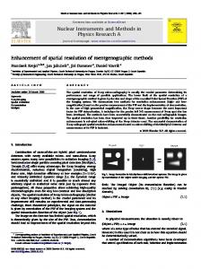
120m Fig. 1. Pixel numbers in the local window at which Band 6 is observed.

Section IV proposes a predictor for Band 6 based on the conditional distribution. Band 6 is corrected by adding a linear combination of high resolution data. The proposed procedure is examined by mean squared errors (MSE's) based on Landsat 5 TM image of Hiroshima City in Section V. Further, Band 6 is enhanced and it is shown that our method reduces the conditional variance into half of the variance of raw data, which means our method provides an accurate predictor for Band 6. Final conclusion is given at Section VII. In the Appendix, we generalize our consideration into a general case. 11.

OBSERVATIONS IN THE

LOCALWINDOW

Consider a local window consisting of 16 pixels of size 120 m x 120 m at which Band 6 is observed. Each pixel is numbered from z = 1 to 16, see Fig. 1. Let xbt be a random variable of Band b at the ith pixel of P the local window. Put

xz = (xlz,x22,

' ' ' 3

x 5 z , x72)'

and

= x6z

where the symbol ' denotes the transposition of the vectodmatrix. In our setup, observations on X, of high resx z z ,. . . ,x5,,m)' are available for olution, say 2, = (xl,, z = 1 , 2 , . . . ,16. On the other hand, each Y, of low resolution is not observed, but the averaged value 5 / 1 6 = y is observed, say 3. Under these conditions, our aim is to predict the values Y, of Band 6 of all pixels based on the observations q ,. . . ,q 6 and in the local window. Fig. 2 gives an example of observed band values in the local window of actual data. Basically, Band 6 is observed once in each local window. Our data is bulk corrected, so y,, corresponding to observed values of Band 6 at zth pixel, are smoothed (resampled) and have small fluctuations.

0196-2892/96$05.00 0 1996 IEEE


1152

expressed by a linear mapping A 2 with a matrix A defined by 38

37

29

28

31

30

29

21

30

26

27

24

35

30

25

27i:

Values of Band 7

0

.. .

A=

0 16

. . .. .. 0 0 1 0

0 0 ,0

24

zli: Values of Band 1

0 0

'I6

0

0

0 0 ..

0 0 ..

I,

0

0 0

1 1

'.. '..

0 0

. .. 0

. * '

1

'

e

'

...

0

: 98 x 112.

(2)

The formulas (1) and (2) show that the joint distribution of A 2 is given by the multivariate normal distribution with mean vector A p and covariance matrix ACA', i.e.,

yi: Values of Band 6

Fig. 2. Band values in the local window. Bands 1 , 2 , 7 are of high resolution, and Band 6 is of low resolution.

111. DISTRIBUTIONS RELATING TO BAND 6

x)',

z = 1, 2, We assume that the random vectors ( X i , ..., 16 are independently distributed as a 7-variate normal distribution with unknown mean vector ( p : ,ut)' and unknown covariance matrix

where 16V = u3. Using the joint distribution (3), we can derive the conditional distribution of YIS as follows. The covariance matrix ACA' appearing in (3) is partitioned as

This distribution is denoted by

where pa:6 x 1. Here, we suppose that C x z : 6 x 6, myy and oxy:6 x 1 are common in the local window. Consequently, the joint distribution of the vector of all band values 2 ( X i ,Y1,.. ,X i 6 , Y 1 6 ) ' : 112 x 1 in the local window is given by the multivariate normal distribution with mean vector p and covariance matrix C , where

oyy- &EF;1J2 l

(5)

= 150yy.,/16

where myu.x is a conditional variance defined by gyy 2

= g y y - o;yc,-,loxy.

(6)

In behalf of the joint distribution (3) and the relations (4) and (5), the conditional distribution of Y 1 6 given X 1 = XI,.. . ,XI6 = X I 6 and = j j is deduced as

N(y + @;,C,-,l(J;16

-

+ 61, x , 15ayy x

/

q

whereI = x,/16: 6 x 1. Here, 516 denotes a difference between two conditional expectations, and is defined for general a by

6%x See, e.g., [6] for the definition and properties of multivariate normal distributions. For simplicity, at first we shall derive the joint distribution of Y16 (unobservable Band 6 at 16th pixel) and of all random vectors whose observations are available. The random vector . . ,xi6, 16u, &)': 98 x 1with 1 6 Y = E:!?l y3 is

(xi, xb,.

= (uz- o;y,x;p,)

-

(v - o;,C,-,1TL)

(7)

where ji = p,/16: 6 x 1. For general i, the conditional distribution of Y, is analogously derived as -

KI(x1 N

=

N(y

+

. ,XI6 = 2 1 6 , Y = ?J} o;yCi2(~c?-I) 5, x , 1 5 c ~ ~ ~ . ~ / (8) 16). '

+

NISHII et al.: ENHANCEMENT OF LOW SPATIAL RESOLUTION

-LOCAL

1153

i.e.,

WINDOW

16

FYY

OXY

where 3 and j j are sample means of high-resolution band values and of band 6 values, respectively. 2) The block estimate +block: Consider a block cdnsisting of 7 x 7 local windows, see Fig. 3. We have essentially 49 observations in the block. First, derive 49 mean vectors of observations on 7 band values obtained in local windows in the block. Next, calculate a sample covariance matrix based on 49 mean vectors which would give an estimate for (1/16) Fig. 3. Block consisting 49 local windows. The sample covariance matrix, calculated by 49 mean vectors of local windows, is used for the enhancement of Band 6 values of the shaded local window.

By virtue of the joint distribution ( 3 ) ,we obtain the conditional distribution of Y , given = j j as

yZl{Y = 7j)

N

N(7j+ V, - V , 15aYy/16).

IV. PREDICTION FOR BAND6 In this section, we will propose a predictor of Band 6 based on the conditional distribution (8). We make the following assumption on the mean vector in each local window. A l ) The difference &.= defined by (7) is sufficiently small. We propose a predictor for Y , by

3 + ~'(z, -I) with 7 = Ei2uZy:6 x 1

Then find an estimate for 7,say +block. 3 ) The global block estimate +g-block : This estimate is similar to.+blockexcept the sample covariance matrix is estimated by mean vectors of all local windows in the whole image. 4) The global estimate +global: The global estimate is also derived by the whole image. Take only one observed 7-variate vector in each local window and calculate the sample covariance matrix. Using the local estimate of 7,the local predictor of Y; are defined by y!ocal

(9)

which is .the conditional expectation in (8). Thus, Band 6 is corrected by the linear combination of high resolution data. Obviously, the predictor in the local window satisfies C,'z,{jj ~'(5, - Z)} = 167j, which is a canonical relation required by the sensor system. The simple predictor 7 j for Y , is derived under the following assumption: A2) The difference v, - V is sufficiently small. Then, its variance is given by 15ayy/16. On the other hand, the conditional variance of ?j 7'(za- I)is given by 15cYyx/16. Therefore, the ratio between the conditional and the unconditional variances is equal to

+

+

Throughout this paper, we assume the assumption Al). The assumption A2) is tight and does not fit for enhancement. A2) is assumed only for the case to consider (10). The prediction formula (9) contains the unknown regression coefficient vector 7 = E ; ~ o , ~ . The following estimates for 7 are obtained when C,,,(T,~ and oYyare supposed to be common locally or globally. 1) The local estimate ?local: The local estimate for the regression vector is given by +local = ?;2bzy, where Ex, and bxy are calculated by the sample covariance based on the 16 observed vectors in each local window,

.

h\

--Y

+ +;oca1 (2,

-

I).

711)

Similarly, according to the estimation methods for 7,weqefine , and pflobal. The local estimate has an advantage that it can be obtained by the data within each local window. However, it is composed by only 16 observations and y; is essentially observed once, so images based on this estimator expected to be unstable. Concerning the block estimate, we use only one mean vector in each local window for estimation. A block size with 3 x 3 local windows would be too small. We choose blocks of size 7 x 7 for the sake'of acquiring a stable estimate for 7.We will return to this point in Section VII. ?:lock,

v.

COMPARISON OF PREDICTORS

The proposed method is applied to Landsat 5 TM image of Hiroshima City, Japan, taken at Oct. 23, 1990. (428 lines x 560 pixels). Figs. 4 and 5 are gray scale images based on Bands 7 and 6, respectively. Again, it is noted that the values of Band 6 are bulk corrected. The performance of predictors (9) with estimates ?block,?g-block, and ?global are examined by using Only is not available high resolution data. (The local estimate in this case.) 1) Discard Band 6 to yield only six full-resolution bands. 2) 4 x 4 average one out of these bands in order to simulate the resolution of Band 6. 3) Predict the low resolution band values by ?:lock, I;;-block, and ?%global.

1154

IEEE TRANSACTIONS ON GEOSCIENCE AND REMOTE SENSING, VOL 34, NO 5 , SEPTEMBER 1996

Fig 4. High resolution TM image based on Band 7 of size 428 x 560 Hiroshima City, Japan at Oct. 23, 1990.

Fig. 5

Low resolution TM image based on Band 6 of size 428 x 56Qt Hiroshima City, Japan at Oct. 23, 1990.

4) Compare MSE’s between predicted and observed values. The MSE’s between predicted and observed values of Band j for j = 1,. . . , 5 and 7 are tabulated in Table I. Columns of Table I: Mean, Block, G-block, and Global denote MSE’s corresponding to in each local window, Y ; l o c k , ?f-block, and Pfloba1, respectively. Table I proves that our predictors work well. Especially, the values of Band 2 are very accurately predicted by other five full-resolution band values. By this experiment, the global predictor shows the best performance and the block predictor comes next. We anticipate that this is true for Band 6.

VI. ENHANCEMENT OF TM BAND6 The image based on the bulk corrected data yz is a little superior to that of 8. Hence, we propose procedures for improving the image by adding linear combinations of fullresolution bands. The following four predictors for Band 6 are corresponding to the estimation procedures for 7,and are applied to the TM data of Hiroshima. The local predictor Yfcal and the block predictor Yzbiock: Define two predictors for Band 6

NISHII et al.: ENHANCEMENT OF LOW SPATIAL RESOLUTION

1155

TABLE I11 SAMPLE COVARIANCE/CORRELATION OF yt AND Xgloba1,SAMPLE SIZE=

Band

1 2 3 4 5 7

Mean

I1

II II

28.50 13.65 36.80 59.57 I 141.69 50.04

I

I

Block

G-block

Global

4.616* 0.748 2.292** 27.767** 17.474* 7.306*

5.935 0.737* 2.636 42.968 17.517 7.441

4.289** 0.702** 2.375* 31.323* 15.776** 6.442**

I

I

I

I

YG 31.2534 0.9632

TABLE I1

Band 3 Band 4 Band 5 Band 7 Band 6 163.095 102.977 250.166 173.884 44.587 110.279 88.289 186.267 121.620 26.504 185.939 152.654 320.829 207.789 43.828 0.567 389.750 487.523 225.855 9.576 0.814 0.855 834.758 456.866 58.812 0.908 0.681 0.942 281.921 48.305 0.576 0.087 0.365 0.516 31.132

Fig. 6. Enlarged low resolution image based on the rectangular region of Fig. 5.

where +local and are the local and the block estimates defined in the previous section. The global block predictor Y:-block: The global block estimate for 7 is given by -&,lock (0.7274, -1.0999,0.1186, -0.1617,0.1228,0.0638). Thus, we propose the global block predictor %g-block - yz

+ 0.7274(~1,- Z1) - 1.0999(~2,

-2

+ 0.1186(23, - 23) 0.1617(~4, + 0.1228(~5, 5 5 ) + 0.0638(%7, -

-

2)

- Z4) -

3 1.5942 34.4279

The global predictor Y;loba1: Sample covariances and correlations calculated by 107 x 140 = 14980 observations selected in each local window are listed in Table 11. If the covariance matrix of (X:, E)’ is common in the whole image, Table I1 yields the global estimate of 7 as (0.3871, -0.3126, -0.0032, -0.0809, -0.0088,0.1489)’. Thus, the global predictor in this case is given by

SAMPLE COVARIANCES/CORRELATIONS OF HIROSHIMA TM IMAGE, SAMPLE SIZE= 14980

Band 1 Band 2 157.020 99.260 0.969 66.831 0.955 0.989 0.416 0.547 0.691 0.789 0.827 0.886 0.638 0.581

239680

ezglob a1

E7). (14)

i/zglobal - yz -

+ O.3871(~1,

- -1)

O.O032(~3,- Z3) 0.0088(~5,- 2 5 )

-

- 0.3126(~2,- Z,)

0.0809(~4,- Z 4 ) - Z7).

+ 0.1489(~7,

(15) To observe in detail, we enlarge the sea and commercial area of Hiroshima. This area of size 100 x 116 is marked in Fig. 5. Fig. 6 is the enlarged image based on yz. This image is enhanced by four formulas (12)-(15) in Fig. 7. The image based on (15) is superior to the other images because the breakwater and roads can be easily detected. Now, the sample covariance and correlation between yz and in the whole image are listed in Table 111. The mean coincides with that of yz. 132.733 of Table I11 shows that the variances of enhanced values are greater than of yz because enhanced values have bigger fluctuations. However, using Table I1 we can estimate the conditional variance (6) as 16.40. This implies that the ratio (10) is 0.526. Thus, our procedure reduces the conditional variance into half of the variance of raw data by using information based on high resolution band data under the assumption A2). Figs. 8 and 9 show the difference betweenpriginal values yz in Fig. 2 and enhanced values Rblock and Kglobal,respectively. It is seen that corrects the raw data yz largely than Rblockdoes. is given Finally, the enhanced whole image based on by Fig. 10.

VII.

CONCLUDING REMARKS

All predictors (12)-(15) for Band 6 are of the form that the raw band 6 value is corrected by the linear combination of high resolution values. Such a correction is theoretically justified. We will summarize their features. 1) The predictors (12)-( 15) satisfy the desirable condition such that the average of enhanced values in the local window is equal to the observation on Band 6. 2) The predictor of the form (9) is simple and unbiased under the assumption Al). Its conditional variance is smaller than the variance of jj under A2).

IEEE TRANSACTIONS ON GEOSCIENCE AND REMOTE SENSING, VOL 34, NO 5, SEPTEMBER 1996

1156

Fig. 7

Enhanced images by four predictors. (a)

Fig. 8. The difference ?:lock

- yz

%local

in (12). (b) %'lock

in the local window used in Fig. 2.

3) The global predictor (15) shows the best performance among four predictors, and the block predictor (13) comes next. The most difficult problem is in estimation of the regression vector 7 because the fluctuations in yt are much smaller than in Y,. The goodness of the global predictor may come from that the predictor is based on the stable estimate +g-block, but +g-block may still estimate 7 downward. The block estimate is fair in this sense because 7 is estimated by the data such that all band values are averaged in each local window. Actually,

in (13). (c)

%g-'lock

in (14). (d)

Fig. 9. The difference ?:lobagl

%gglobal

in (15).

- yz in the local window used in Fig. 2.

f l u c t u a e i n the elements of +g-block given in (14) are bigger than those of (15). The better estimate for mZy would improve predictors, and this problem remains open. We also examined an iterative use of our enhancement procedures. By the numerical example, this procedure behaves like an edging process. However, it is not seen the improvement of MSE's. Thus among four predictors, we recommend the global predictor (15) for Band 6. If the fluctuation in band values in the whole image is big, we expect that the block predictor

NISHII ef al.: ENHANCEMENT OF LOW SPATIAL RESOLUTION

Fig. 10. Enhanced image based on

Rglobal

1157

in (15). Hiroshima City, Japan at Oct. 23, 1990.

works better than the global predictor does. The other problem to find the optimal block size is left for future investigation. Finally, we retum to the normality assumption on 7 band values. Of course, this assumption is too tight in actual data. However, our predictors proposed here still remain useful in the sense that they are linear approximations to predictors based on conditional expectations under nonnormal case.

random vector is derived in the same way by 0 0 0

4 0

0 IP

0 0 0

...

0 0

...

0 0

. . . IP ... 0 ... 0

0 14

0

APPENDIX MORE GENERALSETTING Our treatment in Sections I11 and IV is immediately extended in the general setting. Let random vectors (X:,Y:)’: ( p q ) x 1,i = 1 , 2 , . . . , m , be independently normally distributed as

+

The joint density in the above yields the following conditional distribution of Y , -

Y,I{X1 = 2 1 , . . . , X m = z m , Y=g} N

.. E,,

E,,

E,,

E,, .

0 0

0 0

..’ ... .

.

0 0

.

E,, . . . E,, ” *

0 0

E,, E,,

The special case with p = 6, q = 1, and m = 16 has

Nq(3 + CyzE$(xm

-

z) +

6 2 2 ,

(1 - ~ / m ) C y yz )

wherem:= E,”=,x,:dxl,E,,, = Xyy-X,,X;~EZy: q x q and Sa ,= (v,- EyzE;2pa) - (v - E,,E;;p): q x 1 with mp = C,”=yj: p x 1. If the length of the vector S,, is sufficiently small, we propose the predictor for Y , by ya - y

+

~ y z ~ ~ : (-x 2). a

The unknown matrix CyxE;L: q x p will be estimated locally or globally.

been already considered in this paper. Suppose that observed ACKNOWLEDGMENT vectors x; on X ; are available, whereas the average of Y;’s The authors wish to thank two anonvmous referees for their is only observed as 3: q x 1. Our problem is to predict each careful readings and valuable comments. Their comments led Y , :q x 1by using 5 1 , ’ . ‘ ,xm and 3. Put m y = Y j and mD = CyEl uI.Then, the joint distribution of the following the draft into the drastic revision. Specifically, the referees

*


1158

proposed the block estimate and the comparison of procedures based on the MSE’s. Also, they suggested the iterative use of the enhancement procedures. These points, discussed in Sections IV, V, and VII, respectively, are greatly useful to improve the draft.

Saeko Kusanobu received the B S degree in mathematics from Shimane University in 1994 and the M S degrees in integrated arts and sciences from Hiroshima University in 1996 She is a student of the Graduate School of Engineering, Hlroshima University Her interest includes remote sensing data and ,image analysis based on stahstical techniques

REFERENCES M Inamura, “Improvement of spatial resolution for low spatial resolution thermal infrared image using high spatial resolution visible and near-infrared images,” Trans Inst Electron, Inform, Commun Eng , Part A, vol J 71-A, pp 497-504, 1988 (in Japanese) M Inamura, H Toyota, and S Fujimura, “Exterior algebraic processing for remotely sensed multispectral and multitemporal images,” ZEEE Trans Geosci Remote Sensing, vol 1, pp 112-118, 1982 B Zhukov, D Oertel, and F Lanzl, “A multiresolution multisensor technique for satellite remote sensing,” in Proc 1995 Int Geoscz Remote Sensing Symp , vol I, pp 51-53, 1995 B Zhukov, M Berger, F Lanzl, and H Kaufmann, “A new technique for merging multispectral and panchromatic images revealing sub-pixel spectral variation,” in Proc 1995 Int Geoscz Remote Sensing Symp , VOI 111, pp 2154-2156, 1995 R 0 Duda and P.E Hart, Pattern Classzjication and Scene Analysis. New York Wiley, 1973. C R Rao, Linear Statistical Inference and Its Applications, 2nd ed New York Wiley, 1976, ch 8, Section A

Ryuei Nishii (M’96) received the B.S. degree in mathematics from Nagoya University in 1976 and the M.S. and D.Sc. degrees in mathematics from Hiroshima University in 1978 and 1981, respectively. He was a Research Associate with the Department of Mathematics, Hiroshima University from 1980 to 1985, and moved to the Faculty of Integrated Arts and Sciences of the same university. Presently, he is an Associate Professor in the same faculty He was a Research Scientist with the University of Pittsburgh from 1986 to 1987, and was a Visiting Associate Professor with the Institute of Statistical Mathematics from 1992 to 1993 His current research interests are in the applications of statishcal techniques to remote sensing data and image analysis. Professor Nishii is a member of the Japan Statistical Society, Japan Mathematical Society, and Remote Sensing Society of Japan.

Shojiro Tanaka (M’89) received the M Sc. degree in environmental science in 1986 and the P h D degree (thesis) in environmental planning science in 1992 from Hiroshima University. He was a Research Associate with the Informahon Processing Center, Hiroshima University from 1987 to 1992, and he is currently an Associate Professor with the Department of Computer Science, Faculty of Engineering, Yamanashi University. His interests are in mathematical and statistical modeling of environment, remote sensing, and geometric extension of data models in DBMS. His broad topics converge on one point: actual solution or tool-building for environmental problems. Professor Tanaka is a member of ACM, Japan Statistical Society, Information Processing Society of Japan, Operations Research Society of Japan, and Remote Sensing Society of Japan