by-node models. Thus, simulation scenarios containing several ISP networks become feasible. We introduce a set of suitable analytical network cloud models ...
Enhancing Discrete Event Network Simulators with Analytical Network Cloud Models Florian Baumgartner, Matthias Scheidegger, Torsten Braun University of Bern, IAM, 3012 Bern, Switzerland
Abstract Domains
Discrete event simulation of computer networks has significant scalability issues, which makes simulating large scale networks problematic. We propose to extend the approach by combining it with analytical models for network clouds, which are much more efficient, if less accurate, than nodeby-node models. Thus, simulation scenarios containing several ISP networks become feasible. We introduce a set of suitable analytical network cloud models and also describe how these models can be implemented in the ns-2 simulator using a hot-plug mechanism.
1
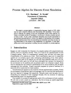
Inter−domain Links
Border Routers
Introduction
Figure 1: The basic modeling view
In traditional packet-based simulators the “world” is modeled in terms of nodes and links with individual capacities and delay characteristics. When simulating whole Internet domains this approach quickly becomes problematic, due to the sheer amount of events to be processed. A multitude of approaches to this scalability problem have been proposed, each with slightly different application ranges. Parallel simulation ([CM81], [ARF99]) is probably the most prominent one, but there are also the approaches of fluid flow simulation ([YG99], [LGK+ 99], [LFG+ 01]), time stepped hybrid simulation [GGT00] and packet trains [AD96], amongst others. A simplified view of the network can significantly reduce the complexity of large scale simulations, but one must give great care to not oversimplify things. Here we propose a model, which we hope will result in far more efficient simulations than traditional approaches but should still give a good approximation of real network behavior. In our modeling view the network is divided into domains and inter-domain links. For each domain, the set of edge nodes and their links to other domains are known, but the topology inside domains is of no concern (i.e. we have a so called black box model). The connections between such domains are modeled by inter-domain link models, which implement properties like link capacity, queuing behavior or Service Level Specifications (SLSs). Figure 1 gives a graphical rendering of this modeling view. Domain and inter-domain link models implement different aspects of network behavior. On one hand, domains are concerned with load distribution, i.e. they model the dependencies between load on the inbound link to the resulting
load on the outbound links. Inter-domain link models on the other hand model the effects these resulting network loads between domains, which are packet loss due to link overload and SLSs enforcement, amongst others. Further components of this model system are the application traffic models concerned with traffic load. They serve to scalably simulate large aggregates of application traffic (VoIP, Video, HTTP, etc.) and their specific properties. Moreover, if these models are derived from network measurements their future properties can be predicted by applying statistical means like ARIMA models. This structure was based on the assumption that congestion is unlikely to occur inside ISP networks since they are usually controlled by a central entity, which can, for example, change the routing to distribute traffic if there is a danger of congestion. In reality this assumption does not generally hold of course, but we expect it to be an acceptable approximation. Since the models described here represent a situation in the real world, measurements from the network are needed to configure them. For traffic load models, these measurements consist of the loads on the inbound links of a domain and their distribution to the outbound links. Furthermore, knowledge of inter-domain topology, inter-domain link capacities and SLSs is required for realistic network modeling. The remainder of the paper is organized as follows: In Sections 2 and 3 we describe the models for domains and inter-domain links, respectively, and Section 4 shows how 1
to combine them to analytical multi-domain models. The integration of these models into ns2 is explained in Section 5. Some preliminary evaluation results are shown in Section 6. Finally, Section 7 concludes the paper.
2
In a simulation scenario the given values are usually the inbound loads. What we would like to have is a so called transit matrix T , so we can write τ11 · · · τ1n .. · I + ε .. (4) Ot = ... t . . t
Domain Model
τm1
where εt is the error term. A way to convert the original result to the transit matrix notation is necessary to accommodate for that. As seen in Equation (2) the inbound load Ij,t is the total of m terms of the form σji Oi,t , for some j. The elements τij of the transit matrix can thus be calculated by σji Oi,t (5) τij = Pm k=1 σjk Ok,t
There are two main aspects to the proposed domain model. One is the traffic matrix describing the dependencies of the load parameters of inbound and outbound links, which is described in the following section. The other aspect is the continuous adaption of this matrix based on measurements done on the live network. It is covered in Section 2.3. As mentioned above the purpose of the domain model is to describe the distribution of traffic flowing into a domain to other domains. We will investigate the scenario where we know two things: the loads on the outbound links at a given time and the origin of these loads by share of the inbound links.
2.1
or, if It is known, by τij =
As mentioned above, we need information about “traffic forking” — the distribution of traffic from an inbound link to the outbound links. Gathering this information from the ingress nodes is not easy in all cases because this might require knowledge of intra-domain topology and routing. It is often easier to determine how much of the load on an outbound link comes from a specific inbound link. As a result we get the outbound loads Ot = (O1,t , . . . , Om,t ) at time t and the relative contributions σji of inbound link j to the load on outbound link i, for every pair (i, j). Thus, the load going from inbound link j to the outbound link i is given by σji Oi,t . Earlier, we stated the assumption that there is only negligible congestion, and therefore packet loss, in a single network domain. We can therefore state that “inbound load = outbound load”, or more formally¿
i=1
Oi,t =
σji Oi,t Ij,t
(6)
given that It 6= 0. Otherwise, we can assume τij = 0. Again, the resulting transit matrix has the property that the element sum of the column vectors equals 1.
Transit Matrix
m X
· · · τmn
n X
Ij,t
2.2
SLSs and Traffic Classes
The transit matrix model discussed above only considers one load parameter per inbound or outbound link. However, there often are several load parameters for various traffic classes defined in service level agreements. Based on the assumption of a “well-behaving network domain” (see Equation (1)) these traffic classes can be considered as independent traffic aggregates. This allows us to describe multiple traffic classes by using one transit matrix per traffic class and domain. Instead of a single transit matrix T the domain model then consists of a set of matrices T1 , . . . , TC where C is the number of separate traffic classes.
(1) 2.3
j=1
Matrix Adaption
Network domains have constantly changing characteristics. Accordingly, a domain’s traffic matrix also changes With this result it follows that the load on a given inbound over time. While the calculation of transit matrices already link j is requires a time series of outbound load vectors and distrim X bution matrices, modeling the changes of domain behavior Ij,t = σji · Oi,t (2) requires a time series of traffic matrices. i=1 From a time series of outbound load vectors Ot and distribution matrices Dt (t = 0, . . .) we thus have to calculate so the whole system can be written as a time series of transit matrices Tu (u = 0, . . .). Let s be the number of observations required to get a good estiI1,t σ11 · · · σ1m O1,t .. .. .. .. (3) mate of the momentary transit matrix of a domain. Then .. . = . . . . the calculation of matrix Tu is based on Ov and Dv where Om,t σn1 · · · σnm In,t v = u · s, . . . , u · (s + 1) − 1. I.e. we make s-sized groups of outbound load vectors and distribution matrices and calculate a transit matrix from each. The sum of elements of the matrix’ column vectors is 1. 2
l1
h1 + q1 l2
domains delay model can be reduced to the simpler formula m X Delay = L + pj
h2 + q2 l3
j=1
where L is constant and pj are poisson distributed random variables. It is important to note that the black box domain model does not allow to store delay characteristics per node in the domain. Each path between two edge nodes must have an own model, include hop count as well as link delay and processing delay characteristics. The adequate model for a path can then be selected by looking at routing information.
h 3 +q 3
Figure 2: General Domain Delay Model Based on this time series of transit matrices we can use several prediction mechanisms like moving average and autoregressive models. However, one problem still remains: The predicted matrices should have the same properties as “real” transit matrices, such as the ones discussed above. Predicting each matrix element in isolation cannot guarantee this. This problem has not been resolved yet and will be a focus of further research.
2.4
3
When choosing an analytical model for inter-domain links, possible alternatives are the traditional queuing theory approach or a fluid simulation approach. While the former may become difficult to calculate in the case of complicated SLSs, the latter may be expected to perform better in such situations but also to yield inferior exactitude.
Domain Delay
3.1
A well-known way of looking at end-to-end delay is to divide it into link, processing and queuing delay. These effects appear in both, domains and inter-domain links. It is a viable approach to build their delay models by deciding whether and how to model these elements of delay. When looking at the case of a path going through a domain it appears clear that all three effects are strongly dependent on the number of hops inside the domain involved. The following formula describes a very general model based on this assumption: Delay =
m X
Inter-Domain Link Model
Fluid Approach
Unlike domain models the inter-domain link model has only one load source, which can usually be described with a single scalar It . If multiple traffic classes have to be distinguished — in DiffServ environments for example — this parameter becomes It = (I1,t , . . . , IC,t ), where C is the number of different traffic classes. The vector elements each describe the bandwidth used by the traffic aggregate of a single traffic class. Models of multiple levels of complexity can be defined based on this input parameter and additional knowledge, such as priorities of traffic classes.
l j + pj + q j 3.1.1
j=1
Here, lj are the link delays, pj the processing delays and qj the queuing delays of hop j. Figure 2 shows this graphically for the case m = 3. The link delays lj are probably not equal to each other but all of them are constant. We can therefore replace these terms in the formula by the constant L. Processing delays on the other hand are not constant and often depend on small timing variations inside the routers. Experiments performed in our testbed have shown that processing delays are approximately poisson distributed. Because we assume that network domains are wellbehaving and congestion only occurs in inter-domain links, queuing delays can only be caused by the burstiness of traffic, which gets smaller the more “backbone characteristics” the domain has. Traffic in backbone domains tends to be smooth because of the great number of microflows it consists of. During validation we will try to show that queuing delays inside domains are really negligible or at least describable by simple means. If the above proves true the
Traffic Class Model Tree
Interrelations between traffic classes can take various forms. Expedited Forwarding for example has absolute priority over other traffic classes, as long as the used capacity remains below a previously fixed value. A more complex example is Assured Forwarding with its three subclasses called dropping precedences, which influence themselves while the whole of them influences other traffic aggregates. I1,t I2,t I3,t
/ µ1 @@ @@ @@ � / µ4 / µ5 / µ2 oo7 o o ooo ooo / µ3 o
/ Ot
Figure 3: Example of a Model Hierarchy Using a model hierarchy these interrelations can easily be modelled. The leaves of this hierarchy tree model the 3
behavior of single traffic classes. Nodes higher in the hierarchy model the interrelations between multiple traffic aggregates below them. Figure 3 shows an example with three leaf nodes and one intermediate node, and of course one root node. In algebraic form the model would read
Dropping Precedences Assured Forwarding (AF) defines three dropping precedences—low, medium and high—which cannot be modelled with the functions above. AF packets are normally marked with low dropping precedence when they are sent and only change that status to a higher dropping precedence if they are detected to be “out of profile” by a router on their path. Then, in case of congestion, routers drop packets with higher dropping precedence first. The following function models a generalized variant of this approach with an arbitrary number of dropping precedences: D1 . ~ , A) ~ = D(B, (b1 , . . . , bn−1 ), M ..
Ot = µ(It ) = µ5 (µ4 (µ1 (I1,t ), µ2 (I2,t )), µ3 (I3,t )) Below a few functions useful to construct such model hierarchies will be defined. In order to make the functions freely combinable they all have to be of a certain algebraic form, which is ~ , A). ~ µ(B, P~ , M (7) Parameter B is the maximum available bandwidth, P~ is a ~ is a vector of n subvector of parameters specific to µ, M ~ models and A is a vector of argument vectors for these sub~ again have the form (P~ , M ~ , A), ~ models. The elements of A although with other vector sizes. The inbound bandwidths Ii,t are considered as constant functions in this context. Furthermore, the following function will help readability:
Dn
Note the parameters b1 , . . . , bn−1 : In contrast to the bandwidth share parameters above they stand for absolute bandwidths. Additionally we assume b1 ≤ B. Again, we need helper functions to describe the elements of the result vector. First, function r calculates the amount of bandwidth m(b, µ, ~a) = min(b, µ(b, ~a)) (8) of a given dropping precedence that has to be retagged to a higher dropping precedence: which according to the above algebraic form can also be � written as max(µ1 (b1 , a~1 ) − b1 , 0) i=1 h(i) = max(µi (bi , a~i ) + h(i − 1) − bi , 0) i > 1 m(bi , µi , a~i ) (12) .. ~ , A) ~ = M (B, (b1 , . . . , bn ), M Using this function we can see how much bandwidth re. mains for a given dropping precedence by m(bn , µn , a~n ) Pn i=1 m(b1 , µ1 , a~1 ) if and only if B ≥ i=1 bi holds. µn (∞, a~n ) + h(n − 1) i = n r(i) = (13) m(b , µ , a ~ ) + h(i − 1) otherwise i i i Fixed Bandwidth Shares The simplest useful function is the one modeling fixed bandwidth shares. Incoming so we can finally write ~ is simply truncated to bandwidth from the models in M � a maximum bandwidth B according to bandwidth shares min(r(1), B) i=1 Pi−1 Di = (14) in P~ = (s1 , . . . , sn ). We get the fixed share function min(r(i), B − j=1 Dj ) otherwise m(s1 B, µ1 , a~1 ) Fair Queueing Fair Queueing and Weighted Fair Queue .. ~ , A) ~ = F (B, P~ , M (9) ing are popular approaches to manage QoS. Our proposed . m(sn B, µn , a~n )
system should therefore provide a rendering of their behavior, or rather just of Weighted Fair Queueing since it is Priority Multi-Queue Multi-queue systems often im- a generalization of Fair Queueing. The parameter vector plement a system of fixed priorities where queues with has again the form P~ = (s1 , . . . , sn ) here. If not all of the small priorities only can send if all queues with higher pri- submodels completely use up their bandwidth share, the ority are empty. This property can be modelled by the func- remaining bandwidth can be used by the other submodels, according to their share. The calculation of the resulting tion bandwidth shares is best done algorithmically. We need m(β(1), µ1 , a~1 ) the following definition: .. ~ , A) ~ = (10) P (B, (), M � . 1, µi (b, a~i ) ≥ b m(β(n), µn , a~n ) α(i, b) = (15) 0, otherwise The name P stands for the priority-dependent behavior of To begin let ι = {1, . . . , n}, W = 1 and b1 = . . . = bn = the function. The helper function β yields the bandwidth 0. The sum of the unused bandwidths of the single flows is available to µi and is defined as calculated by � X B i=1 si si si Pi−1 (11) U = β(i) = α(i, B + bi )( B + bi − µi ( B + bi , a~i )) B − j=1 Pi otherwise W W W i∈ι 4
Then, for every i ∈ ι, reassign � si si α(i, W B + bi ) = 1 W B + bi , bi = si µi ( W B + bi , a~i ), otherwise
Using a P function to combine these, we get the final model Ot = P (100, (), (M, W ), (((25), (I1,t ), ()), A~W )) {z } | M
In the next round only the “unsatisfied” models participate. We reassign ι = {i : i ∈ ι ∧ α(i,
3.2
si B + bi ) = 1} W
Queuing Theory Approach
Traditionally, analytical network models have been based on the queuing theory originating from operations research The sum of weights must also be adjusted, thus we reassign and the like. Although creating such a model for a given X system is often non-trivial, the results are both accurate and W = si efficient. On the other hand, larger systems become very i∈ι complicated to model. From here go to the calculation of U until ι is the empty λ λ set. The variables bi then contain the bandwidths assigned ( & to the models µi . The complete model is then given by @ABC GFED HIJK ONML ... 0 f K g µ µ b1 .. ~ ~ ~ W (B, P , M , A) = . (16) Figure 5: Birth and Death Process bn In the simple case of one queue per inter-domain link we An Example An example should help clarifying the use can use a classic M/M/1/K queue, that is, a queue with exof the above system: Consider an inter-domain link with ponentially distributed inter-arrival time τ and service time the queueing system shown in Figure 4. s, a single “processing station” (the physical link) and a system capacity K. The arrival and service rates are given S EF S by λ = 1/E(τ ) and µ = 1/E(s), respectively. This sys? SSS SSS tem is a birth and death process as shown in Figure 5. For S SS) / / / / a birth and death process of this kind the probability pi of It ? AF Ot WFQ PRIO < ?? y y the system to be in state i is given by ?? y � yy ( BE 1−λ/µ , i=0 1−(λ/µ)K+1 pi = (17) i (λ/µ) p0 , i>0 Figure 4: Inter-Domain Link Example if λ 6= µ, and
Let the total link bandwidth be 100Mbit/s and the bandwidths for the AF dropping precedences be 40Mbit/s, 8Mbit/s and 2Mbit/s, for low, medium and high dropping precedence, respectively. Further, let the WFQ weights be 0.5 for both inputs and 25Mbit/s be the maximum bandwidth allowed for EF traffic. Using the prototypical functions from above we get
p 0 = p1 = . . . = pK =
1 K +1
(18)
if λ = µ. Because here we are only concerned with the changes to the traffic load caused by the queueing system, there is now a very simple way to simulate the dropping behavior. Arriving packets will only be dropped if the queue is full, which is the case with probability pK . It is therefore sufficient to randomly drop an adequate fraction of the arriving packets, or in the case of a input load parameter It to write Ot = (1 − pK )It (19)
M (X, (25), (I1,t ), ()) for the EF queue and D(X, (40, 8, 2), (I2,t , I3,t , I4,t ), ())
for the AF queue (X will be replaced by the function higher in the hierarchy). The Best Effort queue simply uses as Assured Forwarding As mentioned above Assured Formuch bandwidth as it can get, so we can directly take I5,t warding defines three dropping precedences. The differas a model for it. Combining these we get ences in behavior towards these precedences are usually implemented by beginning to drop packets at different fill ~ W (X, (0.5, 0.5), (D, I5,t ), AW ) levels of the queue. This can again be modelled by a birth and death process, although a more complicated one (see for the WFQ queue with Figure 6). The arrival rate λ consist of three rates λl , λm A~W = (((40, 8, 2), (I2,t , I3,t , I4,t ), ()), () ) and λh , for low, medium and high dropping precedence, {z } |{z} | respectively, with λ = λl + λm + λh . The system capacity I D 5,t 5
GFED @ABC 0 f
λ
&
λ
... g
µ
µ
&
GFED @ABC h f
λ−λh
'
λ−λh
...
µ
g µ
'
GFED @ABC m
λl
g
'
λl
...
(
g
µ
µ
ONML HIJK K
Figure 6: AF Birth and Death Process is again K. Medium packets can only be queued if the system contains less than m packets, and high packets only if it contains less than h. The system state probabilities for i > 0 are � �i λ p0 , 0